|
|
Independent Binary Features
As mentioned previously, in pattern recognition
many times a pattern recognition algorithm will output a feature vector
of the observed item. For instance, in the MIT reading machine for the
blind or even the cheque recognition procedure - a feature of d
dimension is output. If each feature in the vector is binary and
assumed (correctly or incorrectly) independent, a simplification of
Bayes Rule can employed:
The 2 Category Case
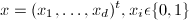
Here, we consider a 2-category problem in which
the components of the feature vector are binary-valued and conditionally
independent (which yields a simplified decision rule):
We also assign the following probabilities (p
and q) to each xi
in X:
 and and 
If pi
> qi, we expect to xi
to be 1 more frequently when the state of nature is w1
than when it is w2.
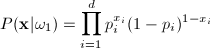
If we assume conditional independence, we can write
P(X|wi)
as the product of probabilities for the components of X. The
class conditional probabilities are then:
Let’s explain the first equation. For
any xi, if it equals 1, then
the expression  is 1. So only is 1. So only  is considered; which makes
sense since pi is the
probability that x=1. If xi=0,
then only the second term is considered, and (1-pi)
is 1 - (probability that x=1)
which is the probability that x=0.
So, for every xi, the
appropriate probability is multiplied to obtain a final product. is considered; which makes
sense since pi is the
probability that x=1. If xi=0,
then only the second term is considered, and (1-pi)
is 1 - (probability that x=1)
which is the probability that x=0.
So, for every xi, the
appropriate probability is multiplied to obtain a final product.
Since this is a two class problem the discriminant
function g(x) = g1(x)
- g2(x)
where:
 and and 
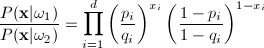
The likelihood ratio is therefore given by:
|
|
which yields the discriminant function as
follows:
|
|
If we notice that this function is linear in xi,
we can rewrite it as a linear function of xi
The discriminant function g(x) will therefore
indicate whether the current feature vector belongs to class 1 and
class 2. It is important to note that w0
and wi are weights
calculated for the linear discriminant. A decision boundary lies
wherever g(x) = 0. This decision boundary can be a line, or hyper-plane
depending upon the dimension of the feature space.
|
|
|
|
The decision boundry
g(x) = 0 is a
line on a cartesian plan for a two dimensional (d =
2) feature space.
|
In a three
dimensional feature space, the decision boundary g(x)
= 0 is a plane,
|
Higher Dimensional Case
Once there are more than two potential classes to classify the data
into, the problem becomes more difficult. The procedure above does not
yield the correct answer since this discriminant function's likelihood
is a ratio between two possible states. Therefore, the discriminant
function shown previously
must be utilized so that every gi( x)
is considered. However, this approach can be used with the following
trick:
- Instead of determining whether the feature
vector belongs to classes {1, 2,
..., n} it is possible to use the above method to
determine the probability that it belongs to class i
or not.
- This is accomplished by setting g1(x)
= gi(x)
and g2(x)=g(not
i)(x). The probabilities for g2(x)
can be obtained by summing all the probabilities for classes {1, ..., i-1
, i+1, ...., n}. If x belongs
to class i, then gi(x)
> g(not i)(x);
otherwise X belongs to some other class.
|
|