Independent Binary Features

As mentioned previously, in pattern recognition many times a pattern recognition algorithm will output a feature vector of the observed item. For instance, in the MIT reading machine for the blind or even the cheque recognition procedure - a feature of d dimension is output. If each feature in the vector is binary and assumed (correctly or incorrectly) independent, a simplification of Bayes Rule can employed:

The 2 Category Case

Here, we consider a 2-category problem in which the components of the feature vector are binary-valued and conditionally independent (which yields a simplified decision rule):

We also assign the following probabilities (p and q) to each x_i in X:

and

If p_i > q_i, we expect to x_i to be 1 more frequently when the state of nature is w₁ than when it is w₂. If we assume conditional independence, we can write P(X|w_i) as the product of probabilities for the components of X. The class conditional probabilities are then:

Let’s explain the first equation. For any x_i, if it equals 1, then the expression is 1. So only is considered; which makes sense since p_i is the probability that x=1. If x_i=0, then only the second term is considered, and (1-p_i) is 1 - (probability that x=1) which is the probability that x=0. So, for every x_i, the appropriate probability is multiplied to obtain a final product.

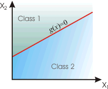
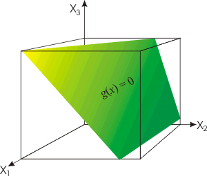
Since this is a two class problem the discriminant function g(x) = g₁(x) - g₂(x) where:

and

The likelihood ratio is therefore given by:

which yields the discriminant function as follows:

If we notice that this function is linear in x_i, we can rewrite it as a linear function of x_i

where

and

The discriminant function g(x) will therefore indicate whether the current feature vector belongs to class 1 and class 2. It is important to note that w₀ and w_iare weights calculated for the linear discriminant. A decision boundary lies wherever g(x) = 0. This decision boundary can be a line, or hyper-plane depending upon the dimension of the feature space.

The decision boundry g(x) = 0 is a line on a cartesian plan for a two dimensional (d = 2) feature space.

In a three dimensional feature space, the decision boundary g(x) = 0 is a plane,

Higher Dimensional Case

Once there are more than two potential classes to classify the data into, the problem becomes more difficult. The procedure above does not yield the correct answer since this discriminant function's likelihood is a ratio between two possible states. Therefore, the discriminant function shown previously must be utilized so that every g_i(x) is considered. However, this approach can be used with the following trick:

Instead of determining whether the feature vector belongs to classes {1, 2, ..., n} it is possible to use the above method to determine the probability that it belongs to class i or not.
This is accomplished by setting g₁(x) = g_i(x) and g₂(x)=g_(not
i)(x). The probabilities for g₂(x) can be obtained by summing all the probabilities for classes {1, ..., i-1 , i+1, ...., n}. If x belongs to class i, then g_i(x) > g_{(not i)}(x); otherwise X belongs to some other class.