Learning Geometric Concepts
Learning Simple Convex Concepts
An algorithm learns a geometric object when it
learns a partitioning of space defined by that object. For example, an
algorithm learns a polygon when it learns a partitioning of the plane in
which the interior of the polygon is labeled with one class and the
exterior is labeled with another.
Observation
1. Under the best-case learning
model, exactly two examples are required by the NN algorithm to learn a
concept by a hyperplane in any number of dimensions.
The strategy of the teacher is to choose any two points
equidistant to the line (or hyperplane) such that the line defined by the
two points is perpendicular to the original. These two points alone will
then correctly classify all future examples. A convex polygon is also very
easy to learn in the best case line ( Figure 2 and 2.1).
|
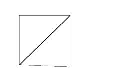
Figure 5
|
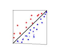
Figure 5.1
|
Learning Complex Geometric Concepts.
Learning complex objects requires some techniques
for learning triangles. Recall the definition of a Voronoi diagram: given a
set of point S. A point is in the Voronoi diagram of S if it is equidistant
to its two NNs (Nearest Neighbors) in S. That is, if a point p has two or
more NNs in S, then p is in the Voronoi diagram of S. Therefore, the
partitioning of space induced by the NN algorithm is, by definition, a
Voronoi diagram.
Observation 2. Suppose we are learning a concept with a triangular boundary.
Suppose also that the triangle is not obtuse: no angles are greater than 90
degree. Then exactly nine points are sufficient for the NN algorithm to
learn the triangle, using the following strategy.
If l is the
length of the shortest side of the triangle, and h is the shortest altitude
of the triangle (the minimum distance of any vertex to its opposite side)
let  =1/2min(l,h). Choose a distance =1/2min(l,h). Choose a distance < < , and place a point this distance from each corner of the
triangle in its interior, such that the point is equidistant from the two
adjacent sides. Then reflect each corner point through the two adjacent
sides. The resulting voronoi diagram defined by the nine points contains
the triangle as a subset. Figure 6 through 7 illustrate such a diagram. , and place a point this distance from each corner of the
triangle in its interior, such that the point is equidistant from the two
adjacent sides. Then reflect each corner point through the two adjacent
sides. The resulting voronoi diagram defined by the nine points contains
the triangle as a subset. Figure 6 through 7 illustrate such a diagram.
|
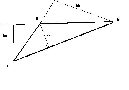
Figure 6
obtaining the shortest distance among the sides and the heights of this
triangle.
|
|
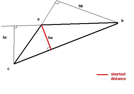
Figure 6.1
Shortest distance is identified with the red line
|
|
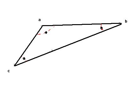
Figure 6.2
red semi-circle representing the distance  from the
corners of the triangle. from the
corners of the triangle.
Figure
6.3 determining the points from each
corners of the triangle and equidistant from the two adjacent sides.
|
|
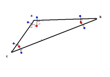
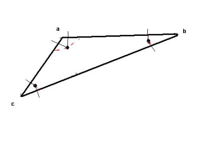
Figure 6.4
blue points obtained through the refrection of the red points with
respects to the adjacent sides.
|
|
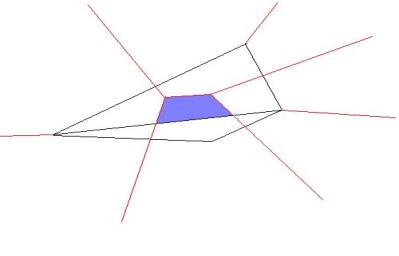
Figure 7 resulting
voronoi diagram
|
The bold lines are the sides of the
triangle; the thin lines are the other edges of the Voronoi diagram. The
intersections of the Voronoi diagram occur on the vertices, edges, and the
interior of the triangle. None of the voronoi diagram occurs outside of the
triangle. This observation applies also to d-dimensional objects in which
all angles between adjacent faces are less than or equal to 90.
|
figure
8 problem with an obtuse triangle
|
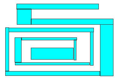
Learning Rectilinear Solids
Theorem1. Any rectilinear polygon with n
edges in two dimensions can be learned in the best-case model with n examples. examples.
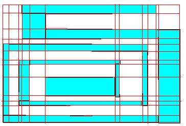
Proof. Draw the smallest possible rectangle
around the rectilinear polygon. For each edge of the polygon, extend the
edge in both directions until it meets the containing rectangle. The
resulting grid contain at most n /4 vertices. Since every vertex of the grid has degree 4,
we can place four points symmetrically around each vertex( arbitrarily
close to the vertex). This set of points will define a Voronoi diagram that
contains the grid, and therefore contains the rectilinear polygon. With
appropriate labeling of points, the learning is complete, having used n /4 vertices. Since every vertex of the grid has degree 4,
we can place four points symmetrically around each vertex( arbitrarily
close to the vertex). This set of points will define a Voronoi diagram that
contains the grid, and therefore contains the rectilinear polygon. With
appropriate labeling of points, the learning is complete, having used n examples. Figure 10 illustrates the grid and the
placement of points for the reclitilinear polygon from figure 9. examples. Figure 10 illustrates the grid and the
placement of points for the reclitilinear polygon from figure 9.
Figure 9 Example of a rectilinear polygon
Figure 10 Learning a rectilinear polygon
|