As we already mentioned in the previous sections, in order to estimate the class-conditional density p(x|X) an assumption is usually made that x|X is distributed normally with unknown parameters. In the framework of this tutorial we'll make another simplifying assumption that the covariance matrix is known.

In this section we'll focus on the case where the feature vectors are one-dimensional. That is, the only parameter in the parameter vector  is the mean . Recall from the approach section that the a priori density of the parameter vector is known. In our case, we'll assume that

that is the mean  is distributed normally with the parameters  and .

Moreover, the parameter vector completely defines the probability density function p(x) which means

where variance is known and mean is the parameter.

Let's now look how to compute p( |X).  It holds that

where n is the number of samples and c₁ is a constant independent of . Since given , p(x|) is distributed normally with the parameters , it holds that

Therefore,

Let's pay attention that

Therefore,

It's easy to verify that p( |X) is also distributed normally, that is

where the parameters  and  depend on the number of samples n. It holds that

where

Now we are ready to compute the desired class-conditional density function:

Therefore, p(x|X) which is equal to the class-conditional density function p(x|w_k,X_k) is normally distributed:

Let's now look at an example illustrating the formulas we developed.

Suppose p(x| )~N( , 4) where p( )~N(0,1). 

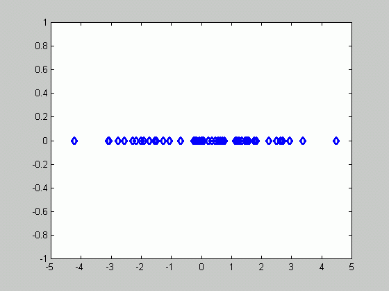
The figure above contains 50 samples.

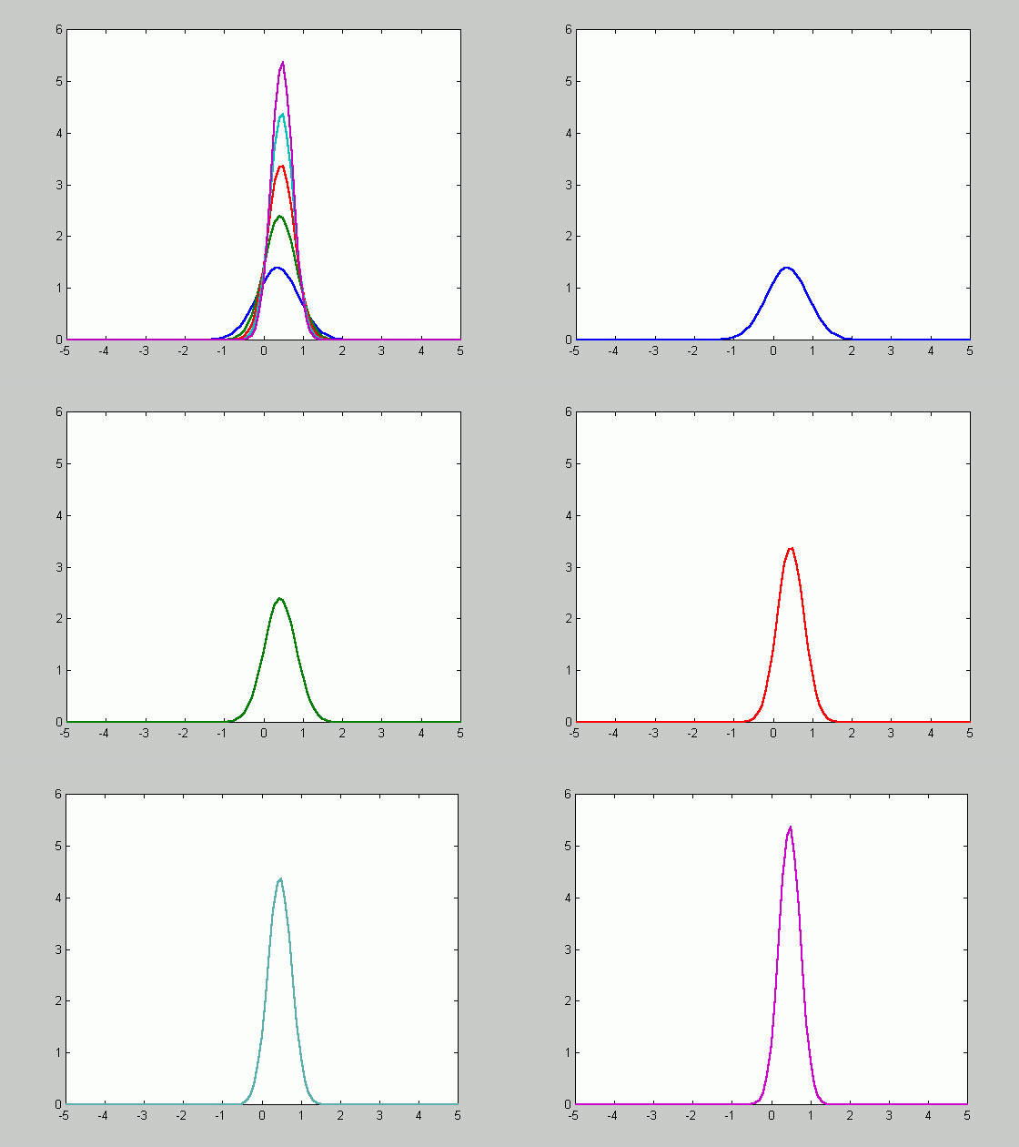
Let's see how p( |X) gets changed as number of samples increases from 10 to 50:

Since  approaches zero as n goes to infinity, the density function gets sharper as the number of samples increases.

Click here to play with an applet illustrating the theory discussed above.