In the previous section we saw how the class-conditional density functions can be estimated in a one-dimensional normal case. Here we'll generalize the ideas and develop the formulas for a multi-dimensional case. The details will be skipped, because the arguments and proofs are quite similar to those in the one-dimensional case.

As before, we'll assume that the p(x|X) is distributed normally and the covariance matrix of the distribution is known. That is the only parameter to be estimated is the mean vector . As in the one-dimensional case, we assume that the unknown parameter is distributed normally with the mean and the covariance matrix . In other words,

To remind you, we are dealing with the multi-dimensional case, so the means and are vectors.

The probability density function p( |X) can be computed by using Bayes rule in the following manner:

where n is the number of samples, is the mean vector and is the covariance matrix. Therefore, p( |X) is also distributed normally:

By equating coefficients it's easy to obtain:

where as before

As for the estimate of the class-conditional density function, it can be computed as before by means of integration:

where

It follows that

In order to illustrate the formulas above, we'll have a look at the two-dimensional case.

Suppose that

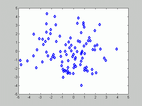
The figure below presents a set of 100 samples.

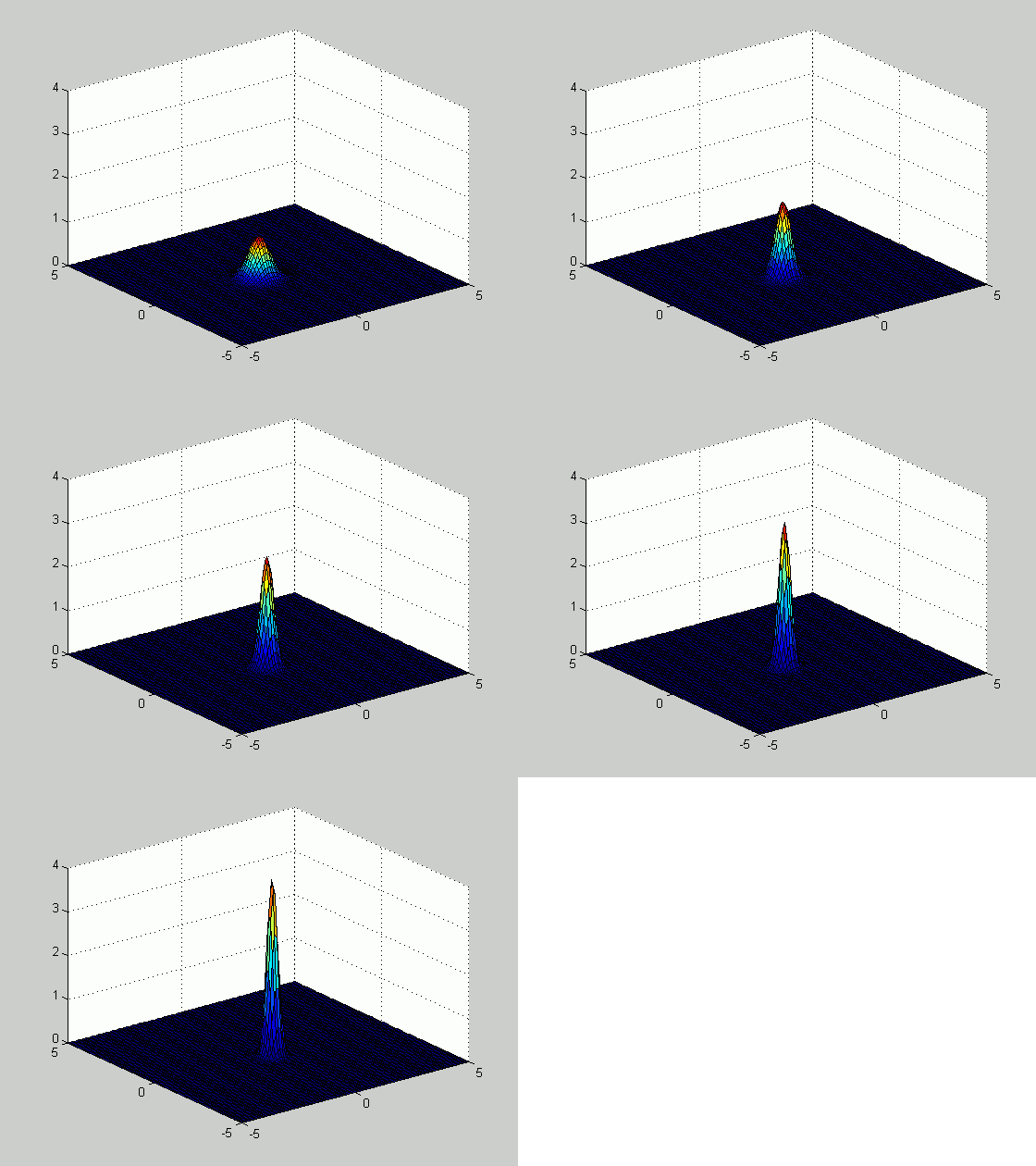
Based on the samples above, we plotted the density function p( |X) as number of samples increased from 20 to 100. The figure below illustrates how the estimated density function becomes sharper as the number of samples increases.