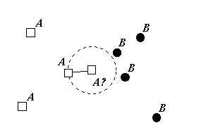
Figure 1.0: The nearest neighbour rule.
Parametric decision rules make the membership classification based on the knowledge of the a priori probabilities of occurrence of objects belonging to some class and the underlining distributions of the probability density functions: which characterise how probable is the measurement should the membership class be .
In many situations, however, these distributions are unknown or are difficult to describe and handle analytically.
Non-parametric decision rules, such as the nearest neighbour rule, are attractive because no prior knowledge of the distributions is required. These rules rely instead on the training set of objects with known class membership to make decisions on the membership of unknown objects.
The nearest neighbour rule, as its name suggests, classifies an unknown object to the class of its nearest neighbour in the measurement space using, most commonly, Euclidean metrics (see Figure 1.0).
Figure 1.0: The nearest neighbour rule.
Beside being extremely simple to implement in practice, the probability of error for the nearest neighbour rule given enough members in the training set is sufficiently close to the Bayes (optimal) probability of error. It has been shown by Cover and Hart [2] that as the size of the training set goes to infinity, the asymptotic nearest neighbour error is never two times worse than the Bayes (optimal) error. More precisely:
Where is Bayes error and is the size of the training set. Furthermore, the performance of the obvious modification for this rule, namely the k-nearest neighbour decision rule, can be even better. The latter classifies an unknown object to the class most heavily represented among its nearest neighbours (see Figure 1.1).
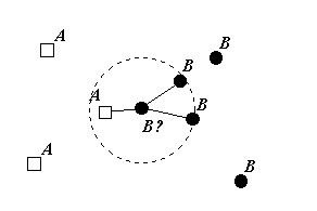
Figure 1.1: The k-nearest neighbour rule.
Despite simplicity and good performance, the traditional criticism of this decision rule pointed at large space requirement to store the entire training set and the seeming necessity to query the entire training set in order to make a single membership classification. As a result, there has been considerable interest in editing the training set in order to reduce its size.
Different proximity graphs (such as Delaunay triangulation) provide efficient geometric apparatus for solving this problem [1].
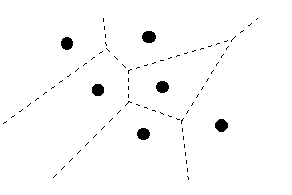
Figure 2.0: Voronoi diagram.
The Delaunay triangulation is a dual of the Voronoi diagram. If two Voronoi regions share a boundary, the nodes of these regions are connected with an edge (see Figure 2.1). Such nodes are called the Voronoi neighbours (or Delaunay neighbours).
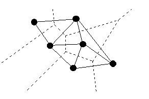
Figure 2.1: Delaunay triangulation.
Considering the nearest neighbour rule, it can be seen that if we compute the Voronoi diagram using the training set as nodes, when some unknown point falls into a particular Voronoi region we must classify this point to the class of that region's node. By definition of the Voronoi region, its every point is closer to the region's node than to any other node, and thus this node must be the nearest neighbour of any new point inside the region.
The decision boundary of a decision rule separates all those points of space in which an unknown object will be classified into some particular class from the remaining points where we classify into some other class. Obviously enough, the decision boundary of the nearest neighbour rule belongs to the Voronoi diagram. In other words, the boundaries of the Voronoi regions separating those regions whose nodes are of different class contribute to a portion of the decision boundary (see Figure 2.2).
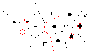
Figure 2.2: The decision boundary.
Although the decision boundary is rarely explicitly computed on practice for high dimension problems, it is clear that, having the decision boundary alone is sufficient to perform the classification of new objects. Hence the nodes of the Voronoi regions whose boundaries did not contribute to the decision boundary are redundant and can be safely deleted from the training set (see Figure 2.3).
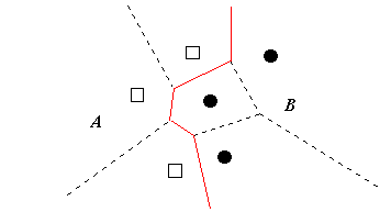
Figure 2.3: The edited training set.
As it can be seen from Figure 2.3, the neighbours of the deleted regions expand, in some sense, to occupy the resulting void.
The above consideration validates the following algorithm for editing the nearest neighbour decision rule:
It is not hard to see, that if there were degeneracies, particularly more than two collinear points, the resulting edited set may not be minimal (see Figure 2.4).
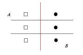
Figure 2.4: A degenerate case.
As Figure 2.4 illustrates, editing will leave all the points, however any two opposite points, one from each class, are enough to preserve the decision boundary.
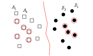
Figure 2.5: Keeping more points than necessary.
As Figure 2.5 illustrates points and are well separated. They are preserved by the Voronoi editing to maintain a portion of the decision boundary. However, assuming that new points will come from the same distribution as the training set, the portions of the decision boundary remote from the concentration of training set points is of lesser importance.
Furthermore, computing the Voronoi diagram in high dimensions is quite costly. Any such algorithm will take in the worst case at least [3] where is the number of points and is the number of dimensions.
The cost of the method and practical necessity to obtain smaller edited sets, lead us to consider some approximate solutions which would be attractive for practical applications.

Figure 3.0: Gabriel neighbours.
As Figure 3.0 demonstrates, the points A and B are Gabriel neighbours, whereas B and C are not.
A graph where all pairs of Gabriel neighbours are connected with an edge is called the Gabriel graph.
The Gabriel editing algorithm can be formulated in a way similar to Voronoi editing:
Although, the resulting Gabriel edited set doesn't preserve the original decision boundary, the changes occur mainly outside of the zones of interest (see Figure 3.1).
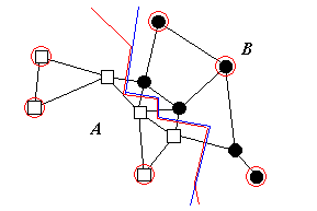
Figure 3.1: Gabriel editing.
Gabriel graph can be computed by discarding edges from Delaunay triangulation. However, the complexity of computing the latter may be as bad as . Thus, this approach is not a very attractive one when number of dimensions is large.
Clearly, the Gabriel graph can be computed by brute force if for every potential pair of neighbours and we just verify if any other point is contained in the diametral sphere:
Since there are potential neighbours and we need to verify every pair by checking other points by using the distance computation which requires steps, the resulting complexity of the brute force algorithm is .
The brute force algorithm can be easily improved by the following heuristic. For a point we create a list of points which are its potential Gabriel neighbours. When checking if the point is indeed the Gabriel neighbour we must perform the test for every point C if it is contained in the diametral sphere (see Figure 3.2).
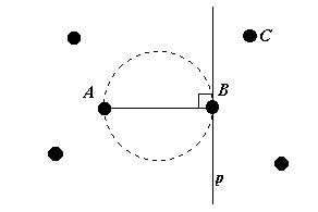
Figure 3.2: Discarding points which can't be Gabriel neighbours.
This heuristic reduces the average complexity to .
Two points and are called relative neighbours, if for all other points in the set, the following is true:
Geometrically, the above implies that no point X is contained in the "lune" constructed on points A and B should the latter be relative neighbours (see Figure 4.0).
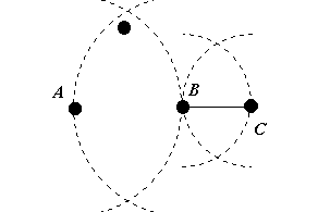
Figure 4.0: Relative neighbours.
As Figure 4.0 demonstrates, the points B and C are relative neighbours whereas A and B are not.
A relative neighbour graph is such a graph where all pairs of relative neighbours are connected by an edge.
Thus, relative neighbour editing algorithm can be expressed similar to Voronoi or Gabriel editing by substituting the relative neighbour graph for the underlining graphs used in those algorithms.
Since the relative neighbour graph is a subgraph of the Gabriel graph, it reduces the size of edited sets even further. However, the changes to the decision boundary can be quite severe, both in the important and less important zones (see Figure 4.1).
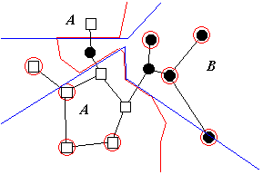
Figure 4.1: Relative neighbour editing.
The algorithm for practical computation of the relative neighbour graph is analogical to that used to obtain the Gabriel graph.