Continuous Bayes Definitions

In the continuous realm, the convention for the probability will be as follows:

where x is a feature vector in d-dimensional space |R^d which will be referred to as feature space; and ω_j represent a finite set of c possible states (or classes) of existence: {ω₁, ..., ω_c}. Note the difference in the above between the probability density function p(x) whose integral

and a probability P(x) represents a probability in the region of [0,1] in which

.

As was stated earlier, the Bayes rule can be thought of in the following (simplified) manner:

The Prior

As the name implies, the prior or a priori distribution is a prior belief of how a particular system is modeled. For instance, the prior may be modeled with a Gaussian of some estimated mean and variance if previous evidence may suggest it be the case. Many times, the prior may not be known so a uniform distribution is first used to model the prior. Subsequent trials will then yield a much better estimate.

The Likelihood

The likelihood is simply the probability of specific class given the random variable. This is generally known and it’s complement is wanted - the a posteriori or the posterior probability.

The Posterior

The posterior or a posteriori probability (or distribution) is what results from the Bayes rule. Specifically, it states the probability of an event occurring (or a condition being true) given specific evidence. Hence the a posteriori is shown as P(ω|x) where ω is the particular query and x is the evidence given.

The Evidence

The evidence p(x) is usually considered a scaling term. Bayes Theorem also states that it is equal to:

therefore, it is also possible to write:

Independence and Conditional Independence

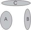
Briefly, it is important to discuss the terms of independence and conditional independence since they figure prominently in the Bayesian world. Independence essentially ensures that two (or more) random variables are not dependent on one another. Graphically, this can be represtented as:

or mathematically by the Joint Probability: P(A,B,C) = P(A)P(B)P(C).

Conditional independence is more relevent to the Bayesian world however. It states that given eveidence, one variable is independent of another. Hence if A ╨ B|C (meaning A is independent of B given C) means that given evidence at C, A is independent of B: