Introduction

A fundamental problem in pattern recognition is that of pattern classification. In many applications, it is necessary to put shapes (patterns) into classes. This is no trivial task; especially if continuous shapes are to be classified. The main problem comes from finiteness --- anything that is done by a digital computer, must be represented in a finite manner. A natural such representation of two dimensional shapes is a finite subset of the shape. These points may be assumed (more often than not) to be uniformly selected from within the shape. In such cases, there is a nice theory that may go a long way toward consistent shape classification. It consists of defining an object called the alpha -hull of the sampled points. It is an inherently ambiguous representation as it involves the tuning of a parameter (alpha). Mandal and Murthy (see [5] ) propose a consistent procedure for selecting this parameter. This page is devoted to presenting their approach.

First, we shall review the fundamental concepts behind alpha-hulls (such as the definition!). An approach for computing them is also provided. Then, the discussion will concentrate on the problem of finding a suitable parameter alpha.

A note to the beginner: Do not let the mathematical notation scare you. When something is stated formally, it is explained in an intuitive way nearby -- either before or after. This approach is used in order to maintain a certain level of completeness while not overwhelming the reader with (largely) unnecessary math scripture.

Alpha-Hulls

Definitions

To define alpha-hulls, we need the notion of a generalized disc. The basic idea behind it is to give a consistent formulation of a disc where the radius may also be negative.

Definition 1. For arbitrary real value alpha , a generalized disc of radius 1 / alpha is defined as follows: Now, we can give the definition of the objects under consideration:

Definition 2.
The alpha < 0  (or alpha-hull) of a planar set S is defined as the intersection of all closed generalized discs of radius 1 / alpha that contain all the points of S. Further, the positive alpha- hull when alpha > 0 . Similarly, the negative hull is for alpha < 0 . Here S will be a finite set of points but, in general, it need not be.

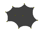
We shall only be interested in the negative alpha -hull. To picture what this is, consider the plane that contains finitely many points S = {X1, X2 , ... , Xn}. Paint it all black. Now, take all the discs of radius 1 / alpha that do not contain any of the points in S, and paint them all white. The resulting shape in black (which will be bounded) is the negative alpha -hull (we picked  alpha < 0 ). See the figure to the right (Figure 1). This process suggests that the as alpha tends toward 0 (i.e. the bigger 1 / alpha gets), the alpha-hull will tend toward the convex hull of S .
ahull-r-35
Figure 1. Example of an alpha-hull.

TRY THIS:
  • Click here.
  • Create points (the set S ) by clicking on the white surface -- try creating the points in Figure 1. 
  • De-select the checkbox "Select -1/alpha" and enter a value for alpha in the text entry beside. Try something between 30 and 100.
  • Click on the button labeled "Compute" and see what happens.
  • You can now change the value of 1/alpha. If you make it 300, the shape you will get is going to be close to the convex hull. However, this requires more memory which may not be available to the applet. Some browsers will simply crash the applet for high values of 1/alpha.


Since we shall not need alpha-shapes here, the reader is referred to Introduction to Alpha Shapes. The page contains a detailed description of the most important notions.

Computation

Here we shall suggest a method for computing the alpha-hull of a planar set of points. It is by no means fancy (or efficient) -- it is easy to understand and implement.

We need the following definition:
Definition 3. Given a planar set (i.e. in R2) of points S = {X1, X2, ... , X n}and a positive real number alpha the alpha -diagram U_alpha of S is the intersection of the 1 / alpha -balls (of radius 1 / alpha ) centred at each point of S, i.e.

U_alpha-eqn .

For negative values of alpha, there is a nice relationship between the alpha-hull and the (-alpha)-diagram. It is stated as the following result:

Proposition 1. Let H_alpha denote the alpha-hull of a set of points S. Further, take U_-alpha to be its diagram. Then

diag-prop .

(See [6, p.16] for a discussion )The important fact from the proposition is that a point in the plane is in the alpha-hull of S only if the ball (disc) centered at that point and of radius abs (1/alpha) is contained in the (- )-diagram of S. In particular, this tells us that the alpha -hull of S is a subset of the (-alpha )-diagram of S . Further, the points in U_-alpha which are not in H_alpha are only those which are less than distance abs(1/alpha) from the boundary of U_-alpha . Hence, the method is

  1. Assume there are finitely many points in S.
  2. Let r = abs(1 / alpha).
  3. Draw black circles (discs/balls) of radius r at each point of S. (This gives the alpha-diagram of S .)
  4. At each point on the boundary of the obtained black region, draw a white (erasing) circle of radius r.
  5. Remaining black region is the alpha-hull of S.

Note that this procedure can be implemented graphically on a discrete grid, such as an image. Simply follow the instructions with this model in mind. However, in this case, the result will only be an approximation of the actual alpha-hull.

Determining Alpha

Alpha-hulls were proposed as a natural generalization of the convex hull of a set of points. They are elegant as one can vary the parameter ( alpha ) and obtain a whole family of hulls. In pattern recognition, an important question is that of how to interpret a set of discrete (finite number) points as a shape. In particular, how to distinguish between different shapes and how to relate similar ones. Mandal and Murthy propose a solution in [5]. The idea is to use the alpha-hull of the set of points and call that the shape. In order to do this, it is necessary to define a procedure for selecting the value of alpha. The purpose of this section is to give such a procedure.

Assumptions

We begin by stating what types of shapes (or pattern classes) will be approximated. Formally, those are assumed to be compact path connected subsets of R 2. This just means that the shapes must be connected, i.e. between any two points in a shape, there must be a trail inside the shape connecting them. Such a pattern class may have wholes but must be bounded.

The problem of assigning a shape to a finite set of points, may be thought of in the following manner. Assume that the points come from an underlying shape. Suppose that they have been picked uniformly at random; that is, every point in the shape is equally likely to have been picked. Now the question becomes: how do we assign a shape to the finite number of points that best approximates the underlying shape ? Even this, however, is ambiguous -- we need to make precise what "best approximates" means. One proposal is to minimize the symmetric difference between the underlying shape and the assigned shape:

Definition 4. Let A and B be subsets of the plane R 2. The symmetric difference, denoted by Delta , is all the points which are in one of the two sets but not in both. Formally, this is

(A intersection complement(B)) union (complement(A) intersection B) .

Definition 5. Let X be a shape (pattern class) and A n the shape assigned to n points selected uniformly at random from X. The shape assignment will be called consistent if the area of the symmetric difference of X and A n converges to 0 as n grows to infinity, i.e. if
symm-diff-estimator .
In other words, the assigned shape must resemble more and more the underlying shape.

The Shape Estimator

We want to define a shape assignment procedure that is consistent according to Definition 5. Consider the following result (explained below):

Theorem 1. Let X be a pattern class according to the assumptions above. Let epsilon_n be a sequence of positive real numbers such that eps_n-to-0 , but where n(eps_n^2) -> infy . Let S = {X1, X2, ... , X n} be point in X selected independently uniformly at random. Then, estimating the shape of S as A n , where
thm1.gif .
is a consistent according to Definition 5.

Proof. Refer to [4].

What the theorem states is that an estimator is consistent if, as n grows, it produces shapes that contain points which are closer and closer to the the points in S. It reflects the intuitive truth that the more points describe a shape the better this description is (more of the shape is covered). However, we do not want the assigned shape to be just the points in S (we would not be gaining anything in such a case). We want them to get closer and closer, but not too fast. This is precisely what the condition n(eps_n^2) -> infy accounts for. Essentially, we want an estimator that accounts for the number of smple points and the scale. Indeed, it is not enough to only consider the number of sample points. It suffices to look at two squares -- one 10x10 and the other 1000x1000 -- to be convinced. (Of course, 100 points may approximate the 10x10 square well but are all too sparse in the 1000x1000.)

Now, if S is as in the theorem, we can take the MST of the points in S. (See the glossary.) Call the minimal spanning length of those points l n and let
h_n .

It can be shown that hn satisfies the properties of  epsilon_n in Theorem 1. (See [7].) Pick alpha according to
alpha = - 1 / h_n

This choice guarantees that the alpha-hull will be a consistent estimate of the underlying shape. For more details, see [5]. Observe, however, that multiplying hn by a constant still satisfies the conditions, that is
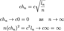
c*h_n still good

A  Note About the Implementation

In the section Computation, we saw how to obtain the alpha-hull of a set of points in the discrete case. However, the criterion for picking alpha outlined in the previous section does not seem to give good results as is. The constant c, as in the last equations, is needed to make the algorithm give reasonable results. This is why, the applet allows the user to select a multiplicative constant c. One does this by entering the value in the text box labeled "alpha scale" (it's initial value is set to 5.0). From the experiments run, and as you can see for yourself playing with the applet, the value of the constant needs to be greater than 1.0. Also, the shapes one obtains with a particular value of c are consistent; that is, the approximated shape (the alpha-hull) converges to the underlying shape as the number of sample points increases. The main reason for having to select this constant is the fact that a circle of radius less than 1.0 cannot drawn properly on a discrete grid.

(All the numbers above are in pixels.)