COMPUTATIONAL GEOMETRY

COMP 507, FALL 2003

THE  UNIMODAL  DISTANCE  FUNCTION  IN  COMPUTATIONAL  GEOMETRY

1. Introduction

2. Defining Distance Functions

3. The Relationship Between Convexity and Unimodality

4. Algorithms

5. Properties of Unimodal Polygons

6. Applet

7. Open Problems

8. References

Introduction

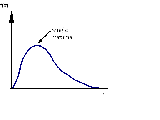
A function f: R-> R is unimodal if it increases to a maximum(minimum) value, and then decreases(increases).

 It is strictly unimodal if it increases and decreases strictly. Essentially what it means is that once the function peaks, then on it's way down, it can't decide to go back up for a bit ever again.

For the purposes of the project, we'll consider polygons unimodal even if the function remains constant over an interval. This makes life easier (well, algorithmically, it doesn't. But we won't go there yet).

 The very concept of UNIMODALITY applies to a number of different fields including probability theory, statistics, and of course, what we’re looking at here, computational geometry.

Introduction  Distance Functions  Relationship  Algorithms  Properties Applet  Open References

Defining the Distance Function

We will be using the Euclidean Distance for all figures and theorems shown here. It is possible to extend this to other metrics including the Minkowski Metric, the Max-Metric etc, but for computational geometry purposes, it is easier to consider only the Euclidean Metric.

 There are 3 cases to deal with:

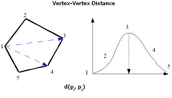
1. Vertex - Vertex Distance :

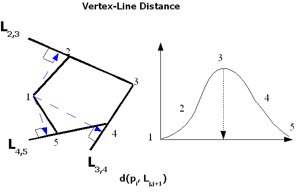
 2. Vertex - Line Distance :

3. Line - Vertex Distance :

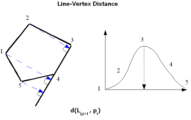
An obvious observation that we make here is that in cases (2) and (3) i.e. VERTEX-LINE and LINE-VERTEX, solving case (2) for all VERTEX-LINE distance pairs is equivalent (computationally) to solving case (3) for all LINE-VERTEX pairs. 

 In general though, we are interested in only case (1)- VERTEX- VERTEX distance.

Introduction  Distance Functions  Relationship  Algorithms  Properties  Applet  Open References and Links

The Relationship Between Convexity and Unimodality

In all the analysis, one question looms above all others. The answer has far-reaching impacts on computational complexities, correctness of algorithms, and generalizations of properties of polygons.

What’s the relationship between UNIMODALITY and CONVEXITY?

-In short, NONE.

We provide examples or rather, counterexamples of different cases of polygons which disprove our premises.

1.    Vertex-Vertex

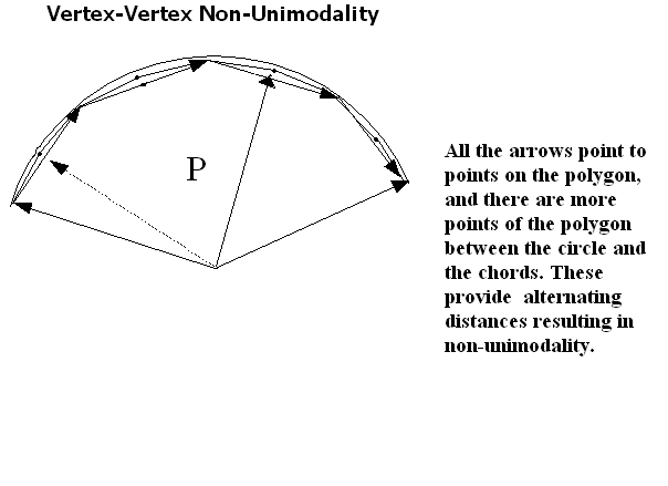
 So is a convex polygon unimodal? – NO

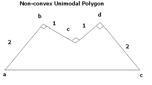
So, is a unimodal polygon convex? - NO

The assumption- CONVEXITY ó UNIMODALITY  is FALSE. This is fundamentally very important, and the assumption of this falsity led to a number of famous diameter algorithms for polygons being incorrect. For more on that, visit a great webpage by another COMP 507 alumnus, Mats Suderman. Go to Diameter Algorithms.

2. VERTEX-LINE

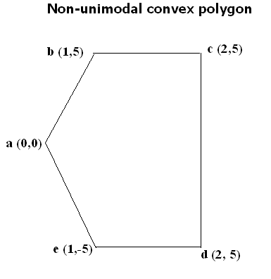
So is a convex polygon unimodal? NO

         The point a here is bimodal with respect to its perpendicular distance from the edges of the polygon P.

   d_a,Li,i+1= {0,5,2,5,0}

But here, we give ourselves hope, a polygon that is f(p_i ^ Lj,j+1) unimodal must be convex. We include the proof in order to show the reader what a proof entails, or rather looks like, because you know how to disprove stuff in Comp Geom., just provide the counterexample.

   Proof:

• Assume P is not convex.

• Then P contains at least one reflex vertex.

• Let p_k be such a vertex.

• Take f(L_k,k+1 ^ p_i).

• We have that Jordan’s Curve theorem => there exist vertices p_i such that d(L_k,k+1 ^ p_i) > 0

•   But, d(L_{k, k+1} ^ ) < 0 since p_k is reflex.

• Also, d(L_k,k+1 ^ p_k) = 0, since p_k is a vertex of the edge.

• Thus,  f(L_k,k+1 ^ p_i) is at least bimodal, and hence not unimodal.

• This provides us with a contradiction.

So finally, to summarize our findings we have the following relationships.

• CONVEXITY ó LINE-VERTEX Unimodality

• Convexity <= Vertex-Line Unimodality

• Convexity ó Vertex-Vertex Unimodality is FALSE

Introduction  Distance Functions  Relationship  Algorithms  Properties  Applet  Open References and Links

The Algorithms:

So now we come to the next important part: determining the modality of a convex polygon.

We of course can consider the Brute-Force algorithm that computes distances between every pair of points in the polygon and checks if the Unimodality property holds or not. We use that in our aplet. But, here we present a more elegant algorithm that is particularly useful with large sets of points.

The following algorithm determines the modality of a convex polygon in time O(n+m), n = |V| , m = modality, reference (3).

It tests whether a convex n-gon is unimodal in q(n) time (proven best possible)

It is also extended to simple polygons – it computes modality of an n-vertex simple polygon in O(n^1.695) time.

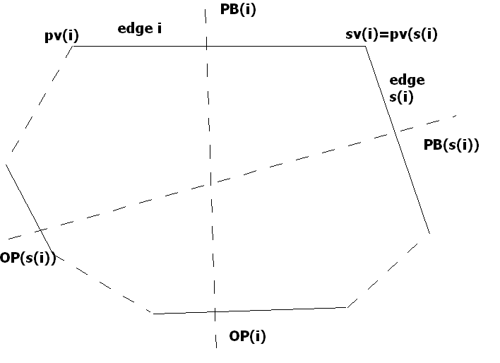
Now for the notation required: 

• s(i)        – successor edge to edge 1

• OP(i)    – edge perpendicularly opposite to edge I

• PB(i)     – perpendicular bisector of edge I

• pv(i)      – previous vertex of edge I

• sv(i)      – successor vertex to edge I

  
  

P is m-modal if the sum of the modalities of the vertices equals m.

The modality of vertex pv(i)  is the number of extremum vertices in the sequence

                            pv(s(i)),  pv(s²(i)), … , pv(s^n-1(i))

sv(j) is an extremum vertex with  respect to pv(i) if either i or ii hold:

i)      d[pv(i), pv(j)] < d[pv(i), sv(j)] > d[pv(i), sv(s(j))]

ii)     d[pv(i), pv(j)] > d[pv(i), sv(j)] < d[pv(i), sv(s(j))]

Algorithm VALGMODAL:

1. Array entry V(i) stores the modality of vertex pv(i) for every edge i of the polygon. Initialize V to zero in O(n) time steps.

2. Compute PB(0) and OP(0) in time O(n). OP(0) is found by scanning at most (n-1) edges to see which one intersects PB(0).

3. (General Step) To simplify notation, we define edge number k to be the edge s^k(0). For 0 <= k <= n-1, compute PB(k) and the intersection of PB(k) with PB(k+1). Note that 2 bisectors must intersect since the polygon is in a given standard form, with no two edges parallel to each other (otherwise the perpendicular bisectors would be parallel too). Determine OP(k+1) by distinguishing between the two cases:

Case 1: Intersection point lies inside the polygon, ie PB(k)intersection PB(k+1) is in between the midpoint of edge k and PB(k)intOP(k). 

Traverse clockwise and check if OP(k), s(OP(k)),…s^j(OP(k)) intersect PB(k+1). 

Let s^j(OP(k)) intersect PB(k+1). 

Then increment the modality of vertices: sv(OP(k)), sv(s(OP(k))),…,(sv(s^j-1(OP(k))) not including sv(OP(k)) if it is the intersection point of PB(k) and OP(k).

            Case 2: The intersection of PB(k) and PB(k+1) lies outside the polygon.

            2.1:  PB(k) intersects edge k+1 between midpoint of edge k+1 and pv(k+1) .             

             Traverse clockwise from k+1 to OP(k+1). Increase the modality of all encountered vertices that are

             not adjacent to:

                    sv(k) i.e. sv(k+2),..,pv (OP(k+1)) but not counting this last vertex if OP(k+1) is edge k.   

             2.2: PB(k+1) intersects edge k between midpoint of edge k and sv(k).  Traverse clockwise

             from OP(k) to edge k and increase modality of all vertices not adjacent to:

              sv(k),…,sv(OP(k)), pv (k-1) not counting the first vertex if OP(k) = edge k+1 or 

              if it is the intersection point of OP(k) and PB(k).

              2.3: Neither PB(k+1) nor PB(k) intersect edge k or edge k+1 respectively as shown (figure d).

              Traverse CCW and check if PB(k+1) intersects any of OP(k), pv(OP(k)),….pv^j(OP(k))) and let  

              pvj(OP(k)) be OP(k+1). 

             Then as in 1, increment modality of: pv(OP(k)), pv(p(OP(k))),…pv(p^j-1(OP(k))) not including the

              last vertex if it is the intersection of PB(k+1) and OP(k+1).

• Since the last two intersection points of PB(k) are known at the beginning of the k-th iteration , the intersection points of PB(k+1) are calculated in O(1). Also, whether or not PB(k+1) or PB(k) intersect each edge k or k+1 respectively takes O(1).

• Thus every iteration of step 3 takes time proportional to the number of vertices whose modality has been incremented.

• Thus overall time for all iterations for an m-modal polygon: O(n+m).

• The algorithm can also be generalized to account for degeneracies, and can be expanded to account for all sorts of polygons, not just simple ones.

Introduction  Distance Functions  Relationship  Algorithms  Properties  Applet  Open References

Properties and Statements:

1. The Nearest Neighbour of every vertex p_i is an adjacent vertex of p_i if P is unimodal.

The corollary also holds:  If a simple polygon P is unimodal, then the closest pair of vertices forms an edge in   PG(P).

2. Define Global Symmetric Furthest Neighbours and Local Symmetric Furthest Neighbour: 

Then if the simple polygon P is unimodal, then every Local SFN pair of vertices of P is also a Global SFN  pair.

3. Unimodality is the property that provides the linearity in the Dobkin-Snyder algorithm. 

4. Algorithms solving the ALL-FURTHEST-NEIGHBOUR problem do so in linear time for convex unimodal polygons.

5. A convex polygon need not contain a single vertex whose distance function f(pi, pj) is unimodal (see Convexity, ...)

Introduction  Distance Functions  Relationship  Algorithms  Properties  Applet  Open References

Applet

Much of the background code for the applet was from S. Legghe's website. Many thanks to him for making it publicly available. It's at: ww.cs.mcgill.ca/~legghe/geo

In order for the relationship to be made clearer between Convexity and Unimodality, the applet allows you to input a convex polygon on the fly and lets you know if it's convex or not.

To the Applet.

Introduction  Distance Functions  Relationship  Algorithms  Properties  Applet  Open References and Links

Open Problems:

1. Can the ALL-FURTHEST-NEIGHBOUR problem be solved in linear time for convex polygons?

2. Given a random convex n-gon, what is the probability that it is unimodal?

Introduction  Distance Functions  Relationship  Algorithms  Properties  Applet  Open References and Links

References:

1. Toussaint, G. T., "Complexity, Convexity and Unimodality" International Journal of Computer and Information Sciences, vol. 13, No. 3, June 1984, pp.197-217.

2. Pach, J., “On an isoperimetric problem”, studia Sci Math Hungary, 13:43-45, 1978

3. Aggarwal, Alok, Melville, R., “Fast Computation of the Modality of Polygons”, Journal of Algorithms, 7,(3): 369-381 (1986)

Links:

COMP 507

Professor: Godfried Toussaint

T.A: Greg Aloupis

The best bar-brewed beer in Montreal is in this bar.

Introduction  Distance Functions  Relationship  Algorithms  Properties  Applet Open  References and Links

Contact: saurja.sen@mail.mcgill.ca . For anything.