In keeping with the notation used in Clarkson's paper, given a Linear Program with n half-spaces, and d dimensions, let S denote the set of n half-spaces. The main ideas that this algorithm uses to solve the linear program are:

The optimal solution to the LP is determined by a subset S^* of S, where |S^*| <= d. So a solution to a linear program with S^* as the set of constraints and d dimensions is the solution to the original problem. So all of the constraints in the set S \ S^* are redundant.
The algorithm attempts to throw away redundant constraints quickly. It does this by building up a set V^* which is a subset of S. After each "succesful" iteration of the body of the algorithm, a set V is added to V^*. V has a few very important properties, it's a subset of S \ V^*, |V| <= 2n^1/2, and it contains at least one constraint of S^*. So after d + 1 successful iterations all of S^* is contained in V^*, and V has size O(dn^1/2). Then for a small set of constraints the the simplex method is applied to find the optimal solution.

The Recursive Algorithm

function x_r^*(S : set_of_halfspaces)
  V^* = {} // the empty set
  C_d = 9d²
  if n <= C_d then return SimplexMethod(S)
  repeat
    choose R subset of S \ V^* at random, |R| = dn^1/2
    x^* = x_r^*(R union V^*)
    V = {H exits in S | x^* violates halfspace H}
    if |V| <= 2n^1/2 then V^* = V^* union V
  until V = {}
  return x^*

A step through the recursive algorithm in 2 dimensions

Suppose you are given the a set of 5 constraints, and your objective was to find the maximum feasible point in the Y direction.

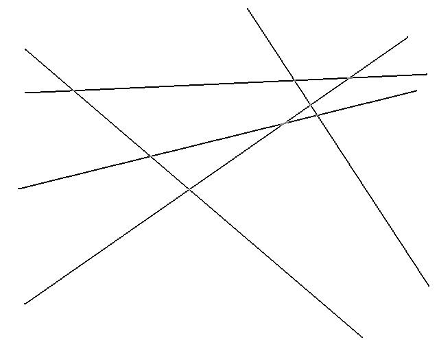
Assume that the feasible region of each half space is below the line in the image.

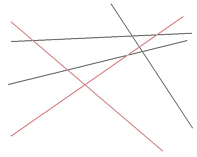
Since d = 2, there are 2 constrains that define the optimal solution. Here we show them in red, they make up the set S^*.

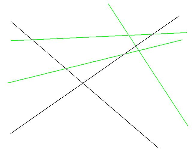
The algorithm begins by selecting a set R randomly from S. The above image shows a possible choice of R in green.

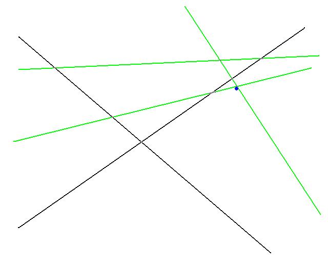
The algorithm would then use the simplex method to find an optimal solution for this set R. The optimal is show in blue above.

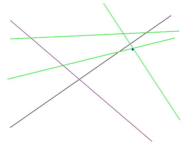
All the constraints that this solution violate are then determined. Here there's only one (the line in purple). The violating constraints are then added to V^*

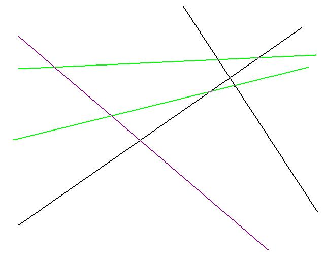
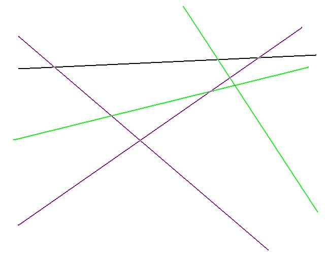
Now a new set R (once again in green) is randomly computed from S \ V^*.

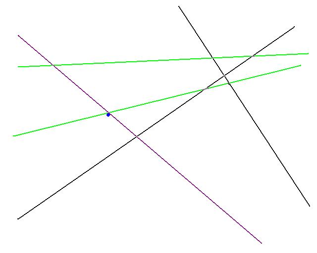
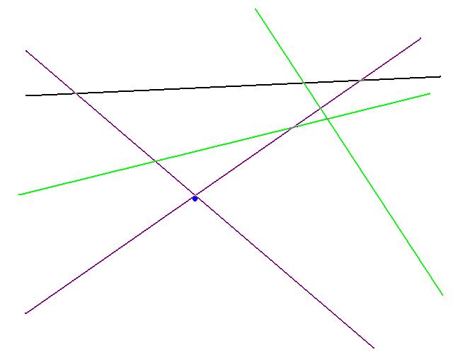
The optimal solution of the LP with constraints R and V^* is then computed. (shown above as the blue dot)

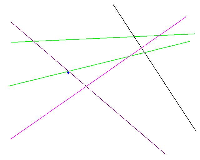
All constraints are checked to see which this optimal violate. They are shown in pink above.

If the number of violating constraints is less then 2n^1/2 then the violating constraints are added to V^*. (Shown in purple above)

A new set of random constraints, R, is picked. An optimal solution is calculated for R union V^*, if no constraint violates this optimal (shown in blue above) we are done. This implies that S^* is contained in R union V^*.