In keeping with the notation used in Clarkson's paper, given a Linear Program with n half-spaces, and d dimensions, let S denote the set of n half-spaces. The main ideas that this algorithm uses to solve the linear program are:

The optimal solution to the LP is determined by a subset S^* of S, where |S^*| <= d. So a solution to a linear program with S^* as the set of constraints and d dimensions is the solution to the original problem. So all of the constraints in the set S \ S^* are redundant.
The algorithm attempts to throw away redundant constraints quickly. It does this by assigning weights to the constraints and choosing a random set of constraints with the probability of being chosen proportional to their weights. The simplex method is then used to compute the optimal value of this random subset. The set of constraints, V, that this optimal value violates is then computed. The weights of these violators is then doubled. Since if V isn't empty it contains at least one element of S^*, it can be show that the weights of S^* increase more rapidly then the weights of other contraints, so eventually with high probability the random set, R, chosen will contain S^* so the optimal will be computed.

The Iterative Algorithm

function x_i^*(S : set_of_halfspaces)
  for H exits in S do w_H = 1 od;
  C_d = 9d²
  if n <= C_d then return SimplexMethod(S)
  repeat
    choose R subset of S at random, |R| = C_d
    x^* = SimplexMethod(R)
    V = {H exits in S | x^* violates halfspace H}
    if w(V) <= 2w(S)/(9d - 1)
	then for H in V do w_H = 2w_H od
  until V = {}
  return x^*

Note: -w(V) = Sum of w_H over all H that exists is V. (similarily defined for w(S))
      -The set R is chosen with probabilities proportional to the elements weights.

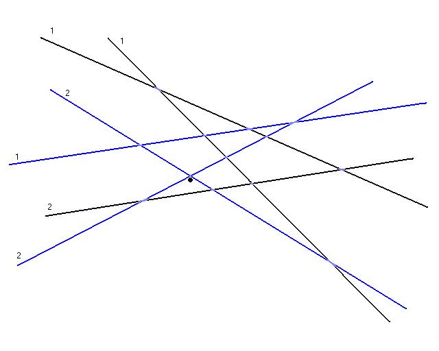
A step through the iterative algorithm in 2 dimensions

Suppose you are given the a set of 6 constraints, and your objective was to find the maximum feasible point in the Y direction.

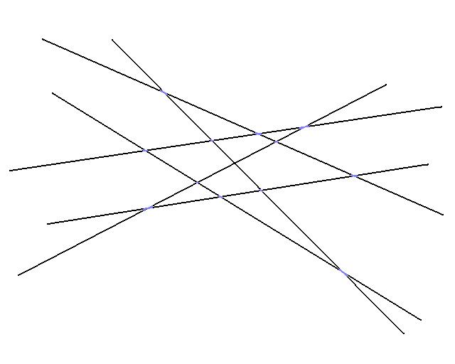
Assume that the feasible region of each half space is below the line in the image.

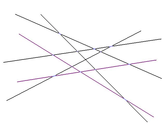
Since d = 2, there are 2 constrains that define the optimal solution. Above we show them in purple above, they make up the set S^*.

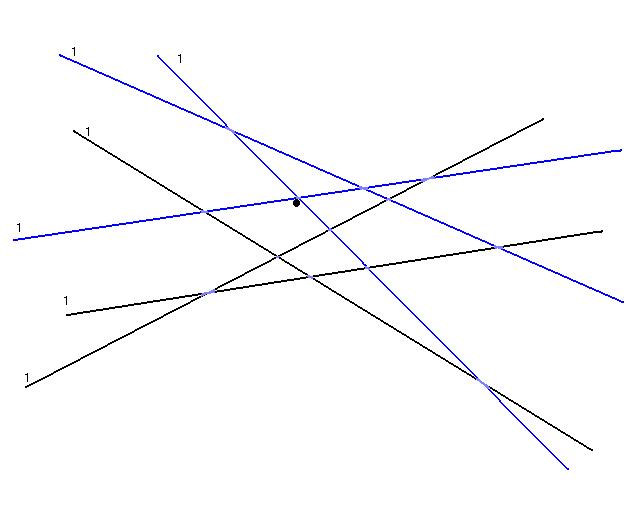
The algorithm begins by selecting a set R randomly from S with probability of being in R proportional to there weights. The above image shows a possible choice of R in blue. The numbers next to the lines denote there current weight. The algorithm would then use the simplex method to find an optimal solution for this set R. The optimal is show as a black dot above.

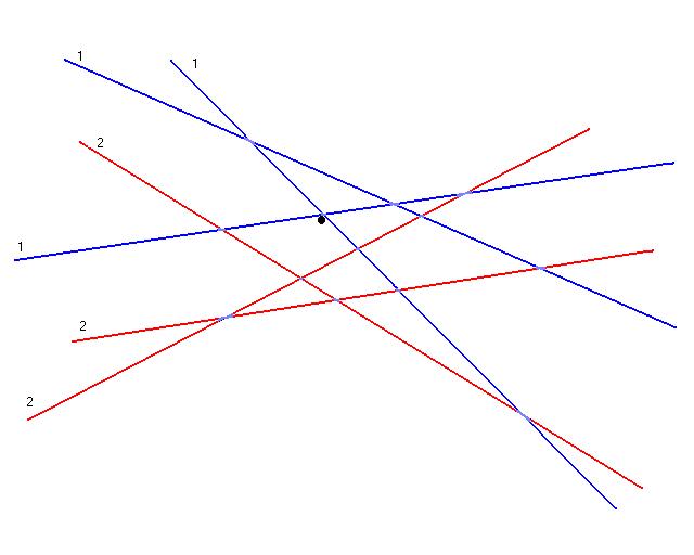
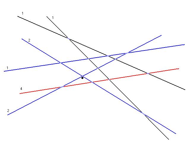
All the constraints that this solution violate are then determined. Here they're shown in red, there weights are then doubled (now they have weights of 2).

Now a new random set, R, of constraints is chosen with probabilities proportional to there weights. Shown above in blue is a possible random choice, now the constraints with weight 2 have a higher probability of being chosen then all the other constraints. Once again the simplex algorithm is used to compute the optimal value for this set of constraints, the optimal is shown as a black dot.

The constraints that the optimal value violates is then computed (once again shown in red). Those constraints weights are then doubled (the weight of 2 becomes a 4).

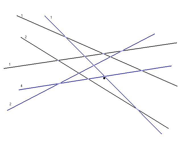
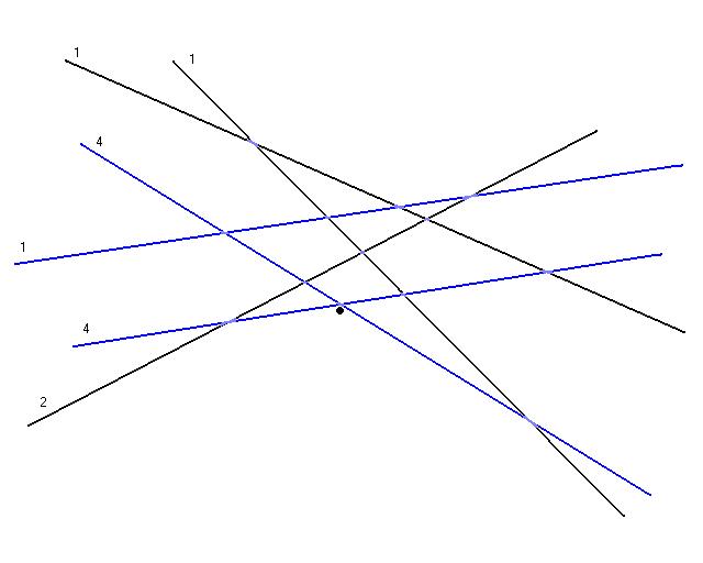
Now a new random set, R, of constraints is chosen with probabilities proportional to there weights. Shown above in blue is a possible random choice. Once again the simplex algorithm is used to compute the optimal value for this set of constraints, the optimal is shown as a black dot.

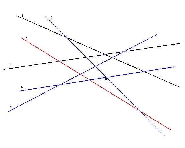
The constraints that the optimal value violates is then computed (once again shown in red). Those constraints weights are then doubled (the weight of 2 becomes a 4).

Once again a random set R is chosen. Now with high probability the choice of R will contain the set S^*, since it's weights are much higher then the weights of the other constraints. The optimal value calculated using the simplex method of this set R doesn't violate any constraints. So this is the optimal value for the linear program and the algorithm terminates.