Genetic algorithms are optimization search methods inspired by the natural process of evolution. From the wing of a butterfly to the fin of a shark, it is observed that nature has come up with an astounding variety of subtle and ingenious solutions to physical optimization problems that still pose a formidable challenge to the modern engineer. So computer scientists have come over to nature's way of thinking. Genetic algorithms seek to replicate the basic components of the nature's evolutionary method: the encoding of organisms as genetic (DNA) data structures, the recombination, mutation and persistence of desirable characteristics, natural selection where only the fittest creatures may survive, the cooperation and competition among the different survival strategies, as well as the ever present role of chance.
The main idea of genetic algorithms is to evolve the best possible solution from random elements.

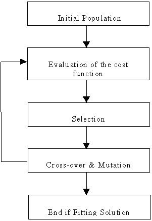
Fig 1 : Scheme of a genetic algorithm
Let's take an example to illustrate the basic principles of genetic algorithms : the search of the maximum of a cost function, which is also called a fitness function.

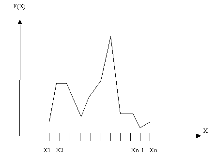
Fig 2: Example of a cost function
A genetic algorithm is working with a set of components, called chromosomes, which are initially randomly chosen in the parameter space. We call this set the population.
We have discretized our parameter space, and we want to find Xmax, which maximizes the cost function F(Xi) over all possible Xi. Each Xi is a chromosome which is encoded as a binary string (hence the discretization of the parameter space), with each bit corresponding to a gene. To solve this problem, we use the scheme described in Fig 1. First, you generate a population. This means that you randomly choose a set of chromosomes in the parameter space : (Xi). Then each point of the population is associated with its cost value, in our case F(Xi). Some points of the population seem better than others. For instance, X2, if chosen, appears better than Xn. We must therefore select the points according to how fit they are, as measured by the cost function. This approach is discussed subsequently and is called selection. We then further explore the parameter space (Xi), in order to improve our solution. Two basic genetic operators are used. First, we use cross-over, and then mutations. At this stage, a new population has been generated which is then tested against the cost function. In this way, we continue searching for the function's maximum. In each generation a new population is created. Others techniques have been developed to hasten the algorithm's convergence and are discussed later. It is difficult to ensure that when we halt the process, our final solution will be indeed a global maximum, and not merely a local one. An appropriate halting criteria must therefore be found. We described this later. At the end of this web page, you will find an applet implementing the example.
The size of the initial population is an important issue because a large population can effectively sample the parameter space. However the larger the population, the higher the computational cost. A compromise must be found. An interesting means to both have an effective sampling and a reasonable computational cost is to decrease the population after the first iteration of the process. For instance, take an initial population of 1000 chromosomes, then choose the 500 better chromosomes and work with this population's size until the end.
The cost function represents the problem we want to solve. For instance, the cost function of the well-known traveling salesman is the distance the salesman has to cover to visit all the towns exactly once. Most search problems may be posed as the search for the optimal value of a function satisfying a set of constraints. The function represents the relationships between the different parameters which we seek to optimize. When those relationships are well-defined and simple enough to be modeled mathematically (e.g. by convex functions), the analytical methods (e.g. Lagrange multipliers) of mathematics should be applied to the problem. When those relationships are so complex as to appear unpredictable or random, the model itself may be ill-posed and only random or exhaustive search offers any hope of an answer. Genetic algorithms are well suited for the real-world problems which lie between these two extremes.
We have now a set of chromosomes. In order to enhance the average fitness of the population, we will generate a new population from the previous one according to the quality of each chromosome: the higher fitness value of a chromosome, the higher its probability to be included in the new generation. The standard way to do this is called the casino roulette method :
Compute ValPop, the sum of all the chromosomes' fitness values :

Then, for each chromosome k, compute its additive fitness value :

Pick at random a number between 0 and ValPop, and choose the first chromosome that has a higher additive fitness value.
You repeat this method until you obtain a population of the desired size.
We now introduce some new information into the population. We use operators that can enhance the evolutionary process by creating new chromosomes from the population.
We first apply an operator called cross-over. It simulates the behavior of DNA: we pick at random two chromosomes named 1 and 2. Then we choose one gene and separate each chromosome in two parts. Finally, we exchange one part of chromsome 1 with the corresponding part of chromosome 2 and vice-versa. Here is an example:
| Chromosome 1 | = | (10010) | Cross-over | (10100) | = | Chromosome 1 | |||||
| Chromosome 2 | = | (00100) | (00010) | = | Chromosome 2 |
The second operator is called mutation. Like in nature, random mutations change the characteristics of the population. You pick at random a chromosome and one of its genes. Then we invert the gene: if its original value is one, we change it to zero; if its original value is zero, its new value becomes one. Here is an example:
| Chromosome 1 | = | (10010) | Mutation | (11010) | = | Chromosome 1 | |||||
| Chromosome 2 | = | (00100) | (00000) | = | Chromosome 2 |
These operators are used to explore of the parameter space once the initial population has been created. At each generation they seek to introduce desirable innovation into the population while hopefully preserving the best of its characteristics. The probability of mutation and cross-over has to be carefully managed to allow the algorithm to converge to a definite, single optimal value.. Too high probabilities prevent convergence, while too low probabilities lead to insufficient exploration of the parameter space to locate a global maximum. We take 70% as a standard probability for cross-over and 8% for mutation.
To allow a faster convergence, some specialized techniques have been developed. We described here two methods. One of these, called elitism, has been implemented in the applet. It is a simple but very powerful idea : we always keep from one generation to another the fittest chromosome. This method enhances greatly the convergence of the genetic algorithm. The other idea tries to improve the efficiency of the operators. It avoids creating any copies of the chromosomes already in the population. If a chromosome generated by an operator has an equivalent one in the population, we apply operator again. This increases the exploration and therefore the efficiency of the operators.
Genetic algorithms are heuristic methods, therefore their halting criterion are also heuristic. The greater the number of generations, the better the solution, until a point is reached when the solution improves no more. To stop when the solution is no longer enhanced is a commonly used halting criterion. Another way is fixing the number of generations. In either case, the best solution found in final population is chosen as the answer.
This little example solve a trivial problem : find the maximum in a an array. However, it is interesting to see the contribution of the different parameters to the algorithm, and its convergence.
This applet is simple to use: with the mouse, select 16 points to define the cost function. You can also choose to pick a random function with the 'Random' button. After the definition of the cost function, the algorithm begins when the button 'Go' is pushed. (The applet requires Java 1.1.).
We have described the basics of genetic algorithms. Lots of methods exist to improve genetic algorithms, like the use of continuous value parameters, where each gene represents a real value parameter instead of a bit of the chromosome's binary string encoding. But the basics remain the same. In our case we want to use genetics algorithms to extract geometric primitives.
Finally lets list some of the key advantages of genetic algorithms:
General, robust approach that can be easily adapted to a wide variety of applications.
Can give a good approximation of the optimal solution even when there are a large number of discrete or continuous parameters.
Capable of optimizing just about any cost function with few, if any, mathematical limitations.
Works well with real-world data.
Suitable to implementation on parallel architectures.