(Under construction)
Copyright: David Avis https://cgm.cs.mcgill.ca/∼avis/
Welcome to the world of Polyhedral Computation. This hands-on guide is meant to be used in conjunction with Komei Fukuda’s Polyhedral Computation FAQ. If you are new to the field and want to find out what it is please click that link now! In fact, most definitions and other theoretical explanations will be given by links to this very useful site. To dive deeper into the theory two excellent resources are Komei Fukuda’s Polyhedral Computation and Günter Ziegler’s Lectures on Polytopes.
We will run almost all examples using the program lrs and a few test files. Most examples can be run directly in your browser by clicking the link run at various places. (Thanks to Yuta Muraya for providing this interface). Note that the input files can be modified and re-run directly in the browser window and this is highly recommended! Alternatively you can download lrs yourself following instructions here and use these input files.
Everyone should at least have the ”hello world” experience by doing Excursion 1. Excursion 2 is a bit technical and boring, but pretty much essential to get any kind of understanding for what is going on. After that most excursions are independent.
Above all this is meant to be a hands on experience, so be sure to run (and modify!) the examples.
A convex polyhedron is defined by a set of linear inequalities and equations. One of the simplest and most useful examples is the 3-dimensional unit cube defined by the inequalities:
It is an example of a bounded polyhedron, or polytope and this representation of it is known as an (halfspace)-representation. Polyhedra can of course be unbounded, but for now we will deal only with polytopes. We will also leave aside for now the possibility of using equations. So an H-representation can be written in the form
where is a column vector of length and is an by coefficient matrix. An inequality that can be deleted without changing the solution set is redundant and the remaining rows after deleting all redundant ones are said to support facets of . Redundancy removal is treated in Excursion 6
It will be represented in lrs by just the table of by coefficients and a few headers. For example the input file contains an H-representation for the cube:
mayumi% cat cube.ine
H-representation
begin
6 4 integer
 0  1  0  0
 0  0  1  0
 0  0  0  1
 1 -1  0  0
 1  0 -1  0
 1  0  0 -1
end
We have a table of coefficients of size 6 by 4 integers which is bracketed by begin and end lines. Each of these rows represents the corresponding row of the matrix .
The Minkowski-Weyl Theorem states every polytope can also be represented as the convex hull of a set of extreme points, its V -representation. The most fundamental task of lrs is to compute a V -representation from an H-representation and vice versa. So let us do it.
The V -representation of the cube is the list of the 8 0-1 vectors of length 3. We can compute
these by running lrs:
(run)
mayumi% lrs cube.ine cube.ext
lrs:lrslib_v.7.3_2023.11.28(64bit,lrslong.h,hybrid_arithmetic)
*Input taken from  cube.ine
*Output sent to file cube.ext

mayumi% cat cube.ext
*lrs:lrslib_v.7.3_2023.11.28(64bit,lrslong.h,hybrid_arithmetic)
V-representation
begin
***** 4 rational
 1  1  1  1
 1  0  1  1
 1  1  0  1
 1  0  0  1
 1  1  1  0
 1  0  1  0
 1  1  0  0
 1  0  0  0
end
*Totals: vertices=8 rays=0 bases=8 integer_vertices=8  max_vertex_depth=3
For simplicity we have deleted a few other lines of output. In the output file the 8 vertices are shown with a leading ”1” that indicates the line gives a vertex (a zero here would indicate an extreme ray, more later). The ”*****” indicates that the number of vertices is not known when the output has started. This is due to the fact that lrs uses the reverse search technique which generates output as a stream, a useful feature for very long runs. The data type is indicated as ”rational” even though all coefficients are integral. Again this is due to the fact the output is generated as a stream. This is our ”hello world” example. If you were able to duplicate this lrs run on your computer, congratulations, everything else will be simple!
If we replace the ”*****” by 8 in
we get a valid V -representation in lrs format. We can run lrs to compute its H-representation:
(run)
mayumi% lrs cube.ext
*Input taken from  cube.ext
H-representation
begin
***** 4 rational
 0  1  0  0
 0  0  1  0
 0  0  0  1
 1 -1  0  0
 1  0  0 -1
 1  0 -1  0
end
*Totals: facets=6 bases=6 max_facet_depth=3
In this case since an output file was not specified the output is produced on the terminal. We find the original 6 halfspaces, albeit in a different order.
This ends our first excursion, we invite you to try out some of the other input files converting from H-representation to V -representation and vice versa.
In Excursion 1 on the *Totals: line you may have noticed the ”bases=n” count. What is a basis? Given an H-representation for a polyhedron in , an extreme point or vertex is defined by a linearly independent subset of inequalities satisfied as equations, whose unique solution satisfies the other inequalities. For example, given rows 1,2,6 give the equations
which has solution that satisfies
the other 3 inequalities. Therefore
is a vertex of .
The set of rows
are called cobasic indices and form a cobasis. The complementary set of rows
are
called basic indices and form a basis. Since bases are in 1-1 correspondence with co-bases we
tend to use the terms interchangeably. By definition, every vertex has a basis. In polyhedral
computation the number of rows is usually much larger than the number of columns, so
printing out the cobasis is usually shorter than printing the basis. There are many
options in lrs (see manual) and most of these are placed after the end statement. In lrs
adding the printcobasis option following the end line does just this. So for example:
(run)
mayumi% lrs cube.ine
printcobasis
V-representation
begin
***** 4 rational
V#1 R#0 B#1 h=0 facets  4 5 6 I#3 det= 1 in_det= 1 z= 1
 1  1  1  1
V#2 R#0 B#2 h=1 facets  1 5 6 I#3 det= 1 in_det= 1 z= 1
 1  0  1  1
V#3 R#0 B#3 h=1 facets  2 4 6 I#3 det= 1 in_det= 1 z= 1
 1  1  0  1
V#4 R#0 B#4 h=2 facets  1 2 6 I#3 det= 1 in_det= 1 z= 1
 1  0  0  1
V#5 R#0 B#5 h=1 facets  3 4 5 I#3 det= 1 in_det= 1 z= 1
 1  1  1  0
V#6 R#0 B#6 h=2 facets  1 3 5 I#3 det= 1 in_det= 1 z= 1
 1  0  1  0
V#7 R#0 B#7 h=2 facets  2 3 4 I#3 det= 1 in_det= 1 z= 1
 1  1  0  0
V#8 R#0 B#8 h=3 facets  1 2 3 I#3 det= 1 in_det= 1 z= 1
 1  0  0  0
end
*Totals: vertices=8 rays=0 bases=8 integer_vertices=8  max_vertex_depth=3
Before each vertex is a line giving its cobasis as a list of facet indices. The cobasis we use above is B#4. The cube has the property that the number of vertices is equal to the number of bases, making it a simplicial polyhedron. Things are not also so nice.
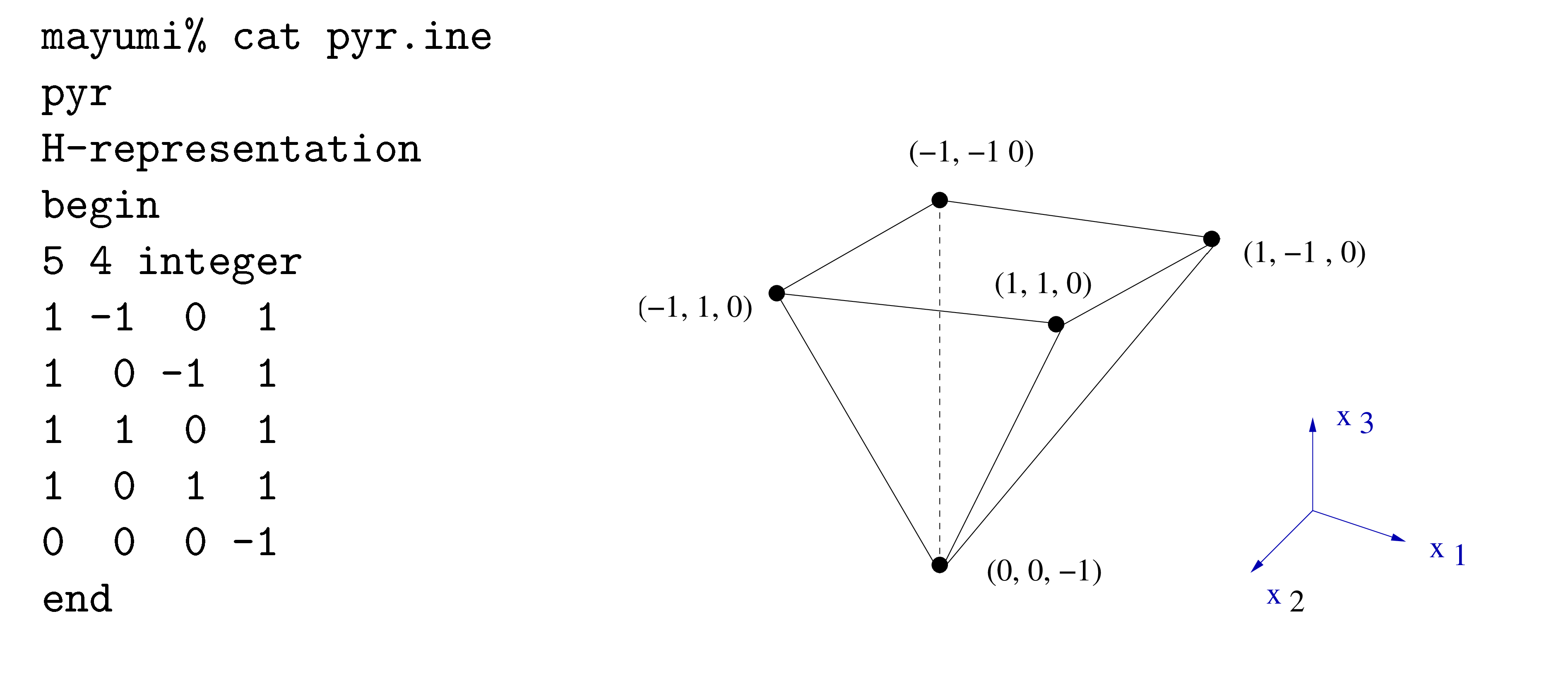
The next example is an inverted pyramid with H-representation
We see from the figure it has 5 vertices. If we run lrs with the printcobasis option we get:
(run)
mayumi% lrs pyr.ine
V-representation
begin
***** 4 rational
V#1 R#0 B#1 h=0 facets  3 4 5 I#3 det= 1 in_det= 1 z= 1
 1 -1 -1  0
V#2 R#0 B#2 h=1 facets  1 4 5 I#3 det= 1 in_det= 1 z= 1
 1  1 -1  0
V#3 R#0 B#3 h=1 facets  2 3 5 I#3 det= 1 in_det= 1 z= 1
 1 -1  1  0
V#4 R#0 B#4 h=2 facets  1 2 5 I#3 det= 1 in_det= 1 z= 1
 1  1  1  0
V#5 R#0 B#5 h=1 facets  2 3 4 I#4 det= 2 in_det= 2 z= 1
 1  0  0 -1
end
*Totals: vertices=5 rays=0 bases=6 integer_vertices=5  max_vertex_depth=2
However this time we see in the *Totals that lrs found 6 bases. Note that the top of the pyramid has
4 vertices, each the intersection of 3 facets, so each vertex has a unique basis. However the apex
is the
intersection of 4 facets and any 3 of these define it. So it has in fact 4 bases representing it. The
normal output of lrs lists each vertex once even if it is represented by more than one basis. To
get lrs to print all bases it discovers we insert additionally the allbases option and now get:
(run)
mayumi% lrs pyr1.ine
V-representation
begin
***** 4 rational
V#1 R#0 B#1 h=0 facets  3 4 5 I#3 det= 1 in_det= 1 z= 1
 1 -1 -1  0
V#2 R#0 B#2 h=1 facets  1 4 5 I#3 det= 1 in_det= 1 z= 1
 1  1 -1  0
V#3 R#0 B#3 h=1 facets  2 3 5 I#3 det= 1 in_det= 1 z= 1
 1 -1  1  0
V#4 R#0 B#4 h=2 facets  1 2 5 I#3 det= 1 in_det= 1 z= 1
 1  1  1  0
V#5 R#0 B#5 h=1 facets  2 3 4 I#4 det= 2 in_det= 2 z= 1
 1  0  0 -1
V#6 R#0 B#6 h=2 facets  1 2 4 I#4 det= 2 in_det= 2 z= 1
 1  0  0 -1
end
*Note! Duplicate vertices/rays may be present
*Totals: vertices=6 rays=0 bases=6 integer_vertices=5  max_vertex_depth=2
The apex is now printed twice giving two of the four bases that represents it. What about the other two bases? lrs avoids generating these vertices by enumerating only a subset of all bases, those known as lexicographically positive. This is an important topic and will be treated in the Excursion on lexicography.
If a vertex can be represented by more than one basis it is called degenerate. Degeneracy can be extremely high: if facets contain a single vertex in then it could have as many as bases. Obviously we only need to find one of basis for each vertex, but no-one has a good way of doing this. For algorithms like reverse search that generate vertices by generating bases, high degeneracy is indeed the villain. Solutions involve using large scale parallelization, as in the mplrs wrapper for lrs or using a completely different method, such as the double description method discussed in another Excursion. Finally we note that a V -representation may be degenerate also and this is discussed in Excursion 5
If we delete the inequality from the unit cube we get an unbounded polyhedron which is the cube with its ”top” cap removed. is the H-representation:
mai6% lrs cube2.ine
H-representation
begin
5 4 rational
 0  1  0  0
 0  0  1  0
 0  0  0  1
 1 -1  0  0
 1  0 -1  0
end
printcobasis
Computing the V -representation with the printcobasis option (see Excursion 2) we get:
(run)
mai6% lrs cube2.ine
printcobasis
V-representation
begin
***** 4 rational
V#1 R#0 B#1 h=0 facets  3 4 5 I#3 det= 1 in_det= 1 z= 1
 1  1  1  0
V#1 R#1 B#1 h=0 facets  3* 4 5 I#2 det= 1 in_det= 1 z= 1
 0  0  0  1
V#2 R#1 B#2 h=1 facets  1 3 5 I#3 det= 1 in_det= 1 z= 1
 1  0  1  0
V#3 R#1 B#3 h=1 facets  2 3 4 I#3 det= 1 in_det= 1 z= 1
 1  1  0  0
V#4 R#1 B#4 h=2 facets  1 2 3 I#3 det= 1 in_det= 1 z= 1
 1  0  0  0
end
*Totals: vertices=4 rays=1 bases=4 integer_vertices=4  max_vertex_depth=2 vertices+rays=5
We now have the 4 vertices of the cube on the plane plus the extreme ray, indicated by a zero in the first column, (0,0,1). Any point in can be expressed as a convex combination of the 4 vertices plus a non-negative scale of (0,0,1). Turning to the cobasis listing, the 4 vertices are expressed as the intersection of 3 input inequalities satisfied as equations, as we saw in Excursion 2. The extreme ray is output as:
V#1 R#1 B#1 h=0 facets  3* 4 5 I#2 det= 1 in_det= 1 z= 1
 0  0  0  1
This indicates that it can be expressed as the intersection of inequalities 4 and 5 satisfied as equations,
ie and
, and bounded by inequality
3 (indicated by 3* ), ie. .
The extreme ray follows the vertex to which it is attached in the output listing.
Note that the extreme ray could also have been expressed as the intersection of
, or
or
. There
are 4 parallel rays in the geometric figure. lrs with the geometric option will list all the geometric
rays.
(run)
mai6% lrs cube2a.ine
printcobasis
*geometric
V-representation
begin
***** 4 rational
V#1 R#0 B#1 h=0 facets  3 4 5 I#3 det= 1 in_det= 1 z= 1
 1  1  1  0
V#1 R#1 B#1 h=0 facets  3* 4 5 I#2 det= 1 in_det= 1 z= 1
 0  0  0  1
V#2 R#1 B#2 h=1 facets  1 3 5 I#3 det= 1 in_det= 1 z= 1
 1  0  1  0
V#2 R#2 B#2 h=1 facets  1 3* 5 I#2 det= 1 in_det= 1 z= 1
 0  0  0  1
V#3 R#2 B#3 h=1 facets  2 3 4 I#3 det= 1 in_det= 1 z= 1
 1  1  0  0
V#3 R#3 B#3 h=1 facets  2 3* 4 I#2 det= 1 in_det= 1 z= 1
 0  0  0  1
V#4 R#3 B#4 h=2 facets  1 2 3 I#3 det= 1 in_det= 1 z= 1
 1  0  0  0
V#4 R#4 B#4 h=2 facets  1 2 3* I#2 det= 1 in_det= 1 z= 1
 0  0  0  1
end
*Note! Duplicate rays may be present
*Totals: vertices=4 rays=4 bases=4 integer_vertices=4  max_vertex_depth=2 vertices+rays=8
In the output there are 4 parallel geometric rays, all with direction (0,0,1) and following the vertex to which they are attached. lrs will normally not report parallel rays and gives a message when this is a possibility.
An important case of an unbounded polyhedra are cones. Here the vector is all zeroes. An important example relates to finite metrics which can be viewed as weighted complete graphs whose edge weights satisfy the triangle inequality. Specifically, let the edge weights of be represented by variables . Given the triangle inequality can be written
gives us a set of triangle inequalities which define the metric cone . For we have 12 triangle inequalities:
mai6% cat m4.ine
H-representation
begin
12 7 rational
 0 -1  1  0  1  0  0
 0  1 -1  0  1  0  0
 0  1  1  0 -1  0  0
 0 -1  0  1  0  1  0
 0  1  0 -1  0  1  0
 0  1  0  1  0 -1  0
 0  0 -1  1  0  0  1
 0  0  1 -1  0  0  1
 0  0  1  1  0  0 -1
 0  0  0  0 -1  1  1
 0  0  0  0  1 -1  1
 0  0  0  0  1  1 -1
end
Let us find the V -representation:
(run)
mai6% lrs m4.ine
*Input taken from  m4.ine
V-representation
begin
***** 7 rational
 1  0  0  0  0  0  0
 0  1  0  0  1  1  0
 0  0  0  1  0  1  1
 0  0  1  0  1  0  1
 0  1  1  0  0  1  1
 0  1  1  1  0  0  0
 0  0  1  1  1  1  0
 0  1  0  1  1  0  1
end
*Totals: vertices=1 rays=7 bases=10 integer_vertices=1  max_vertex_depth=1 vertices+rays=8
The output indicates one vertex, the origin, and 7 other lines indicating extreme
rays. Note that these are all 0/1 vectors so we can interpret them as subgraphs of
. The first ray indicates the star
and the fourth ray indicates
the bipartite graph . In fact the
output consists of all cuts in and
is known as the cut cone. For
the cut cone and metric cones are identical, but this is not the case for
. For example,
for ,
contains all
cut vectors in
plus and additional class of extreme rays.
(run)
mai6% lrs m5.ine
*Input taken from  m5.ine
V-representation
begin
***** 11 rational
 0  0  1  0  0  1  0  0  1  1  0
 0  1  1  1  0  0  0  1  0  1  1
 0  1  1  2  1  2  1  2  1  2  1
.....
end
*Totals: vertices=1 rays=25 bases=573 integer_vertices=1  max_vertex_depth=8 vertices+rays=26
We can turn the cut cone into the cut polytope by changing the
vector to all ones, converting extreme rays into extreme points.
Similarly we can obtain the metric polytope from the metric cone. For
the V -representation of
the cut polytope is denoted
and its H-representation can be computed by lrs:
(run)
mai6% lrs cp4.ext
H-representation
begin
***** 7 rational
 2 -1 -1  0 -1  0  0
 2  0 -1 -1  0  0 -1
 2 -1  0 -1  0 -1  0
 2  0  0  0 -1 -1 -1
 0  0 -1  1  0  0  1
........
 0  1  1  0 -1  0  0
end
*Totals: facets=16 bases=4 max_facet_depth=1
In addition to the 12 triangle inequalities defining we find 4 new triangle inequalities. This is also the H-representation of the metric polytope .
You are invited to investigate these two cones in directories ../ine/metric and ../ext/cut in the lrslib-073 distribution. The essential reference for cuts and metrics is Deza and Laurent’s Geometry of Cuts and Metrics.
In Excursion 1 we noted that equations can be used in an H-representation as well as inequalities. Of course any equation can be expressed as two inequalities but there are various reasons why it is better to express them explicitly. Returning to the cube, we can consider the system:
In lrs format the input file can be written:
lcube
H-representation
linearity 1 5
begin
5 4 rational
 0  1  0  0
 0  0  1  0
 1 -1  0  0
 1  0 -1  0
 1  0  0 -1
end
The first 4 input rows give the inequalities and the fifth gives the equation. Applying lrs to compute
a V -representation:
(run)
lg% lrs lcube.ine
V-representation
begin
***** 4 rational
 1  1  1  1
 1  0  1  1
 1  1  0  1
 1  0  0  1
end
The output gives the 4 vertices of a square located on the plane .
For another simple example consider the line represented by the H-representation :
line
H-representation
linearity 1 1
begin
1 3 integer
1 -1 -1
end
We compute the V -representation:
(run)
line
V-representation
linearity 1  1
begin
***** 3 rational
 0 -1  1
 1  1  0
end
Now we have a linearity in a V -representation which describes the line as
Next we we turn to the travelling salesman problem. If we have four cities labelled then there are three tours: 12341, 13241, 12431.
Using variables these can be coded as 0/1 vectors of length 6. In lrs format we have the V -representation :
tsp4
V-representation
begin
3 7 integer
1 1 0 1 1 0 1
1 1 1 0 0 1 1
1 0 1 1 1 1 0
end
What is the H-representation?
(run)
lg% lrs tsp4.ext
H-representation
linearity 4  1 2 3 4
begin
***** 7 rational
-2  1  1  1  0  0  0
-2  1  1  0  1  0  0
 0  0 -1  0  0  1  0
 0 -1  0  0  0  0  1
 1 -1  0  0  0  0  0
-1  1  1  0  0  0  0
 1  0 -1  0  0  0  0
end
*Totals: facets=3 bases=1 linearities=4 facets+linearities=7 max_facet_depth=0
The output contains 4 linearities which (up to row operations) are equivalent to the degree constraints indicating that a tour must use two edges for each city:
The H-representation is rounded out by the three inequalities:
These seem surprisingly unsymmetrical given the symmetry of the problem. This is due to the
linearities. Indeed if we subtract the first linearity from the first inequality we get the equivalent inequality
. If we subtract the
second linearity we get .
This illustrates a problem created by linearities: the H-representation is not
unique. To get a unique H-representation we need to use the linearities to remove
variables from the problem. Adding the extract option to the H-representation
and
running lrs:
(run)
lg% lrs tsp4a.ine
*switching to extract mode
*extract 0
*extract col order: 1 2 3 4 5 6
H-representation
begin
3 3 rational
 1 -1  0
-1  1  1
 1  0 -1
end
*columns retained: 0 1 2
lrs has eliminated one variable for each linearity. The user can specify which ones to eliminate but the default is to eliminate from the highest column index to the lowest. The output shows that the H-representation of in terms of variables and is
plus the above displayed 4 linearities.
We should caution that the extract option does not necessarily give a minimum representation as an H-representation may contain hidden, ie. not explicitly stated, inequalities. This is the subject of Excursion 7.
To delve deeper into the travelling salesman problem there is nowhere better than Bill Cook’s home page.
Computing the volume of a polytope is a notoriously difficult problem. One way to do this if you have a V -representation is to use lrs with the volume option. Adding this to we obtain the additional output line
*Volume=1
as expected. To see how lrs computes the volume we need to return to the topic of bases and
cobases introduced in Excursion 2. Let us insert the volume, printcobasis and allbases options to
. getting
We
now get output:
(run)
mayumi% lrs cube1.ext
lrs:lrslib_v.7.4_2025.6.20(64bit,lrslong.h,hybrid_arithmetic)
*Input taken from  cube1.ext
cube1
*volume
printcobasis
*allbases
H-representation
begin
***** 4 rational
F#0 B#1 h=0 vertices/rays  4 6 7 8 I#8 det= 1 in_det= 1 z= 1
F#1 B#1 h=0 vertices/rays  4 6 7* 8 I#4 det= 1 in_det= 1 z= 1
 1 -1  0  0
F#2 B#1 h=0 vertices/rays  4 6* 7 8 I#4 det= 1 in_det= 1 z= 1
 1  0 -1  0
F#3 B#1 h=0 vertices/rays  4* 6 7 8 I#4 det= 1 in_det= 1 z= 1
 1  0  0 -1
F#3 B#2 h=1 vertices/rays  4 5 6 7 I#8 det= 1 in_det= 1 z= 1
F#4 B#2 h=1 vertices/rays  4* 5 6 7 I#4 det= 1 in_det= 1 z= 1
 1  0  0 -1
F#4 B#3 h=2 vertices/rays  3 4 5 7 I#8 det= 1 in_det= 1 z= 1
F#5 B#3 h=2 vertices/rays  3 4 5* 7 I#4 det= 1 in_det= 1 z= 1
 1  0 -1  0
F#6 B#3 h=2 vertices/rays  3 4* 5 7 I#4 det= 1 in_det= 1 z= 1
 0  1  0  0
F#6 B#4 h=3 vertices/rays  2 3 4 5 I#8 det= 1 in_det= 1 z= 1
F#7 B#4 h=3 vertices/rays  2 3 4 5* I#4 det= 1 in_det= 1 z= 1
 0  0  0  1
F#7 B#5 h=4 vertices/rays  1 2 3 5 I#8 det= 1 in_det= 1 z= 1
F#8 B#5 h=4 vertices/rays  1 2 3 5* I#4 det= 1 in_det= 1 z= 1
 0  0  0  1
F#9 B#5 h=4 vertices/rays  1 2* 3 5 I#4 det= 1 in_det= 1 z= 1
 0  1  0  0
F#10 B#5 h=4 vertices/rays  1 2 3* 5 I#4 det= 1 in_det= 1 z= 1
 0  0  1  0
F#10 B#6 h=2 vertices/rays  2 4 5 6 I#8 det= 1 in_det= 1 z= 1
F#11 B#6 h=2 vertices/rays  2 4 5* 6 I#4 det= 1 in_det= 1 z= 1
 1 -1  0  0
F#12 B#6 h=2 vertices/rays  2 4* 5 6 I#4 det= 1 in_det= 1 z= 1
 0  0  1  0
end
*Unscaled volume= 6
*Volume= 1
*Totals: facets=12 bases=6 max_facet_depth=4
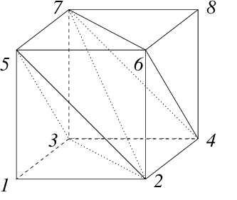
Since we used the allbases option some facets may be produced more than once due to degeneracy (see Excursion 2). In this case each facet is output twice, hence we get 12 facets instead of 6 without the duplication. Each new basis is accompanied by a list of indices representing vertices in the input file. To be a cobasis these vertices are affinely independent representing a simplex. The full set of 6 cobases decomposes the cube into 6 simplices:
2 4 6 7, 4 6 7 8, 2 3 4 7, 2 5 6 7, 2 3 5 7, 1 2 3 5
as shown in the figure.
On each cobasis line printed we find ”in_det=1” which indicates the determinant of the current basis matrix. This determinant is times the volume of the simplex. Since lrs has computes the decomposition of the cube into simplices the sum of the 6 determinants divided by gives the volume of 1. A general discussion of the theory behind this can be found here.
We can also obtain a triangulation of the surface of the polyhedron from the printcobasis listing. We see that the first cobasis 2 4 6 7 generates the facet F#1, 1 -1 0 0, ie. , with cobasis 2 4 6 7*. Deleting the starred index 7* we see that F#1 is spanned by the vertices on rows 2,4,6 of the input , ie. (1,0,0), (1,1,0) and (1,0,1). when index 7* is deleted. The second cobasis 4 6 7 8 generates 3 facets with cobases 4 6 8, 4 7 8, 6 7 8.
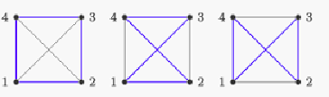
In the full output each of the 6 facets of the cube appears twice corresponding to two triangles:
2 4 6, 4 6 8, 6 7 8, 4 7 8, 3 4 7, 2 3 4
5 6 7, 2 5 6, 3 5 7, 1 3 5, 1 2 3, 1 2 5
Together these 12 triangles triangulate the boundary of the cube, as can be verified in the figure.
The repetition of facets in the allbases listing is how degeneracy appears in a V -representation. In a non-degenerate V -representation each facet is a simplex and appears once. Such a polyhedron is called simplicial. The triangulation produced by lrs corresponds to a deformation of the cube into a simplicial polytope. Note that this is the analog of the cobases generated in an H-representation to V -representation computation corresponding to the vertices of a simple polytope, after deformation in case of degeneracy.
As an example using volumes we return to the cut and metric polyhedra
we met in Excursion 3. As we noted, the extreme points of the cut polytope
are a subset of those
of the metric polytope .
So we may wonder how much bigger the latter is? We can compute the volume of each by
including the volume option:
: (run)
:
(run)
mai6% lrs mp5.ext
*volume
H-representation
begin
***** 11 rational
 0  0  0  0  0  0  0  0  1 -1  1
 0  0 -1  1  0  0  0  0  1  0  0
.......
 0  0  0  0  0  0  1  1  0  0 -1
 0  1 -1  0  0  1  0  0  0  0  0
end
*Volume=4/1701
*Totals: facets=40 bases=14108 max_facet_depth=12

mai6% lrs cp5.ext
*volume
H-representation
begin
***** 11 rational
 2  0  0  0  0  0  0  0 -1 -1 -1
 2  0  0  0  0  0 -1 -1  0  0 -1
.......
 2 -1 -1  0  0 -1  0  0  0  0  0
 6 -1 -1 -1 -1 -1 -1 -1 -1 -1 -1
end
*Volume=32/14175
*Totals: facets=56 bases=124 max_facet_depth=4
We can calculate that cp5 has volume 96% of the metric polytope mp5. In general, optimizing over the cut polytope, the max-cut problem, is NP-hard whereas it can be done by linear programming in polynomial time over the metric polytope (since the H-representation has a cubic number of inequalities).
In Excursion 3 we discovered the metric cone which gives all the distances, known as semi-metrics, on a give finite set. Most people learn that distances are non-negative and satisfy the triangle inequalities. However we did not specify non-negativity in the H-representation . Let us do this getting . It just requires us to append an identity matrix.
lg% cat m4n.ine
m4
H-representation
begin
18 7 rational
 0 -1  1  0  1  0  0
 0  1 -1  0  1  0  0
.....
 0  0  0  0  1 -1  1
 0  0  0  0  1  1 -1
 0  1  0  0  0  0  0
 0  0  1  0  0  0  0
 0  0  0  1  0  0  0
 0  0  0  0  1  0  0
 0  0  0  0  0  1  0
 0  0  0  0  0  0  1
end
When we run lrs we obtain the same V -representation as we did with
:
(run)
lg% lrs m4n.ine
V-representation
begin
***** 7 rational
 1  0  0  0  0  0  0
 0  1  1  1  0  0  0
 0  0  1  1  1  1  0
 0  1  0  0  1  1  0
 0  0  1  0  1  0  1
 0  1  0  1  1  0  1
 0  0  0  1  0  1  1
 0  1  1  0  0  1  1
end
*Totals: vertices=1 rays=7 bases=68 integer_vertices=1  max_vertex_depth=3 vertices+rays=8
This indicates that the non-negative inequalities are redundant, ie. they can be deleted without changing the output. However there is a big difference in the length of two calculations. The Totals line we obtained in Excursion 3 when running lrs on was:
*Totals: vertices=1 rays=7 bases=10 integer_vertices=1 max_vertex_depth=1 vertices+rays=8
This has the same number of vertices and rays, but bases=10 versus bases=68 for the redundant representation . Methods like lrs enumerate bases and the running time is proportionate to their number (see Excursion X on degeneracy). So the running time increases by a factor of about 7. This is a tiny problem, but if we look at the same Totals for and we get respectively:
lg% lrs m5.ine
.......
*Totals: vertices=1 rays=25 bases=573 integer_vertices=1  max_vertex_depth=8 vertices+rays=26

lg% lrs m5n.ine
......
*Totals: vertices=1 rays=25 bases=5197 integer_vertices=1  max_vertex_depth=10 vertices+rays=26
Now 9 times as many bases are enumerated, so things are getting worse. Clearly it is important for large problems to eliminate any redundancy before doing the lrs run. This can be achieved by using the program redund in the lrslib-073 distribution, or adding a redund option after at the end of the input file. The format of the option is
redund i j
which checks lines
in the input file for redundancy, and removes any redundant ones giving a new H-representation. Without
specifying
and
the entire input file is checked. After inserting redund at the end of the input file
we
obtain
and running lrs:
(run)
lg% lrs m4nr.ine
*switching to redund mode
*redund  1 18
*checking for redundant rows only
H-representation
begin
12 7 rational
 0 -1  1  0  1  0  0
 0  1 -1  0  1  0  0
..............
 0  0  0  0  1 -1  1
 0  0  0  0  1  1 -1
end
*input had 18 rows and 7 columns
* 6 redundant row(s) found
 13 14 15 16 17 18
*no check for hidden linearities
This is the original H-representation and this output can be piped back into lrs to obtain the V -representation .
lg% lrs m4nr.ine |lrs
V-representation
begin
***** 7 rational
 1  0  0  0  0  0  0
 0  1  0  0  1  1  0
 0  0  0  1  0  1  1
 0  0  1  0  1  0  1
 0  1  1  0  0  1  1
 0  1  1  1  0  0  0
 0  0  1  1  1  1  0
 0  1  0  1  1  0  1
end
*Totals: vertices=1 rays=7 bases=10 integer_vertices=1  max_vertex_depth=1 vertices+rays=8
Note that only 10 bases are enumerated in the second step, as expected. The message about ”hidden linearities” will be discussed in Excursion Y.
A more general form of the redund command is
redund_list
which instructs lrs to check the input line numbers with indices and remove any redundant lines.
In general checking redundancy is much faster than computing an H-representation to V -representation conversion, so if there is any doubt redundancy should be eliminated.
Adding redund or redund_list options to an input file puts lrs into redund mode. If redund is a link to lrs then
mai6% redund filename
performs the same function as adding redund as an option.
Although it is best to specify linearities directly in the input file they may appear
implicitly in an H-representation by having an inequality and its negation. For example,
is
with the negation
of the first row, ie.
added as a 7th inequality. Together the make the linearity
.
However if we do a redund check by adding the redund option and running lrs we get:
(run)
mayumi% lrs cube4.ine
*redund  1 7
*checking for redundant rows only
H-representation
begin
6 4 rational
 0  1  0  0
 0  0  1  0
 0  0  0  1
 1  0 -1  0
 1  0  0 -1
 0 -1  0  0
end
*input had 7 rows and 4 columns
* 1 redundant row(s) found
 4
*no check for hidden linearities
lrs has eliminated the now redundant
but did not locate the hidden linearity. This is because the (legacy) operation of redund does not
look for them! To do this it is necessary to insert a new (from lrs v.7.3) option testlin before the
begin line.
(run)
mayumi% lrs cube4.ine
*testlin
*redund  1 7
*hidden linearities exist
H-representation
linearity 1 1
begin
5 4 rational
 0  1  0  0
 0  0  1  0
 0  0  0  1
 1  0 -1  0
 1  0  0 -1
end
*input had 7 rows and 4 columns
* 2 redundant row(s) found
 4 7
* 1 hidden linearity found
*minimum representation : dimension=2
In this case lrs first performs an LP to determine if hidden linearities exist. If so, each input line is first checked to see if it is redundant and if so it is eliminated. If it is not redundant a second LP is used to check if it is a linearity. If so the two inequalities are replaced by a single linearity. At the end of the run all linearities are printed first, after eliminating any linearly dependent ones. Since the remaining rows do not contain linearities or redundancies, the output is minimum in terms of the number of rows in the H-representation. A minimum representation can greatly speed up an H-representation to V -representation conversion or a projection (see Excursion 8) and so is highly recommended.
In the presence of other linearities, even explicit ones, hidden linearities can be hard to find. For example, can you find a hidden linearity in this input derived from that we encountered in Excursion 4?
tsp4b
testlin
H-representation
linearity 4  1 2 3 4
begin
8 7 rational
-2  1  1  1  0  0  0
-2  1  1  0  1  0  0
 0  0 -1  0  0  1  0
 0 -1  0  0  0  0  1

-1  0  1  1  0  0  0
-1  1  1  0  0  0  0
-1  0 -1  0  0  1  1
 1  0 -1  0  0  0  0
end
redund
We label the variables as edges of
as before. If you subtract the first linearity (row 1) to the first inequality
(row 5) you obtain 1 -1 0 0 0 0 0 corresponding to the inequality
.
Similarly if you add the third and fourth linearities from row 7 you get -1 1 0 0 0 0, or
. Hence the
hidden linearity
exists in the input file. Running lrs in minrep mode we get the same result:
(run)
tsp4b
*testlin
*hidden linearities exist
H-representation
linearity 5 1 2 3 4 5
begin
7 7 rational
-2  1  1  1  0  0  0
-2  1  1  0  1  0  0
 0  0 -1  0  0  1  0
 0 -1  0  0  0  0  1
-1  0  1  1  0  0  0

-1  1  1  0  0  0  0
 1  0 -1  0  0  0  0
end
*input had 8 rows and 7 columns
* 1 redundant row(s) found
 7
* 1 hidden linearity found
The new inequality is obtained from the original row 5 and is which is equivalent to .
To just find out if an H-representation or V -representation contains hidden linearities one can just add the testlin option but not the redund option to the input file. Adding testlin and redund inequalities to an input file puts lrs into minrep mode. If minrep is a link to lrs then
mai6% minrep filename
performs the same functions without the need for options.
An important operation in manipulating polyhedra is projection to lower dimensions. lrs projects a polyhedron onto a subset of its variables by use of either the project or eliminate options. The former option has the form:
project
This asks for the projection of the polyhedron onto the variables corresponding to columns Column indices are between 1 and and column zero is automatically retained. Alternatively we can specify which columns to eliminate:
eliminate
This eliminates variables corresponding to columns by projection onto the remaining variables. They are eliminated in the order given.
These computations are easy for a V -representation but potentially very difficult
problem for an H-representation. For a V -representation it is a matter of extracting
the required columns and then removing redundancy. Adding project 2 1 3 to
we
obtain
and running:
(run)
mayumi% lrs cube.ext
*switching to fel mode
*project 2  1 3
*removing redundant rows
V-representation
begin
4 3 rational
 1  1  1
 1  0  1
 1  1  0
 1  0  0
end
*columns retained: 0 1 3
These are the 4 vertices of the unit square. There is no search for hidden linearities, so if this is required the input file should be pre-processed or post-processed in minrep mode, described in Excursion 7.
Given an H-representation the projection problem is considerably more complicated. lrs solves this by using the Fourier-Motzkin elimination method.
Variables not contained in the list are eliminated using a heuristic which chooses the column which minimizes the product of the number of positive and negative entries. Redundancy is removed after each iteration using linear programming. Adding project 2 1 3 to modification of we obtain
mayumi% cat cube6.ine
cube6
H-representation
begin
7 4 rational
 0  1  0  0
 0  0  1  0
 0  0  0  1
 1 -1  0  0
 1  0 -1  0
 1  0  0 -1
-1  0  0  1
end
project 2 1 3
and doing a lrs run we obtain:
(run)
cube6
*switching to fel mode
*project 2  1 3
*after removing column 2
*checking for redundant rows only
H-representation
begin
4 3 rational
 0  1  0
 1 -1  0
 1  0 -1
-1  0  1
end

*original vars remaining: 1 3
Note that the input has a hidden linearity in lines 6 and 7, so the output is . A similar result is produced by the option eliminate 1 2. The output as a valid lrs input file.
It is preferable to remove any hidden linearities and redundancy before projection by pre-processing the input file in minrep mode, as described in Excursion 7. Using preprocessing and a pipe we get:
mayumi% minrep cube5.ine | lrs
*hidden linearities exist
*finding minimum representation
H-representation
linearity 1 1
begin
3 3 rational
 1  0 -1
 0  1  0
 1 -1  0
end
*input had 4 rows and 3 columns
* 1 redundant row(s) found
 4
* 1 hidden linearity found
Projection is a useful operation for combinatorial polytopes. We saw in Excursion 3 that all extreme rays
of the metric cone
can be expressed by 0/1 vectors, but this is not the case for
.
If we project out any variable, corresponding to an edge
in
, from
we get the metric
cone for the graph .
This can be computed by inserting eliminate 1 1 to the input file getting
and
running lrs to get:
(run)
*switching to fel mode
*eliminate 1  1
*after removing column 1
*checking for redundant rows only
H-representation
begin
21 10 rational
 0 -1  1  0  0  0  0  1  0  0
 0  1 -1  0  0  0  0  1  0  0
 0  1  1  0  0  0  0 -1  0  0
..................
 0  0  0  0  0  0  0 -1  1  1
 0  0  0  0  0  0  0  1 -1  1
 0  0  0  0  0  0  0  1  1 -1
end

*original vars remaining: 2 3 4 5 6 7 8 9 10
Applying lrs again we see that all extreme rays are 0/1 valued. This can be done in one step by use
of a pipe:
(run)
mayumi% lrs m5.ine | lrs
V-representation
begin
***** 10 rational
 1  0  0  0  0  0  0  0  0  0
 0  1  0  0  1  0  0  1  1  0
 0  0  0  1  0  0  1  0  1  1
 0  1  1  0  0  0  1  0  1  1
 0  1  1  1  0  0  0  0  0  0
 0  0  1  1  1  0  0  1  1  0
 0  0  0  1  1  1  0  0  1  1
 0  0  1  0  0  1  0  1  0  1
 0  1  1  0  1  1  0  0  1  1
 0  1  0  1  0  1  0  1  0  1
 0  0  0  0  1  1  1  0  0  0
 0  1  0  0  0  1  1  1  1  0
 0  0  1  1  0  1  1  1  1  0
 0  0  1  0  1  0  1  1  0  1
 0  1  0  1  1  0  1  1  0  1
end
*Totals: vertices=1 rays=14 bases=100 integer_vertices=1  max_vertex_depth=2 vertices+rays=15
The observant reader will have noticed that these extreme rays are cut vectors and that the cut set with vertices is missing. This is because it gives a redundant cut vector, being the sum of cut vectors generated by the sets . In fact a theorem of Barahona and Mahjoub says that the metric cone of any graph without a minor is the same as its cut cone. See, e.g., Deza and Laurent’s Geometry of Cuts and Metrics.
In closing we should remark that once hidden linearities have been removed from the input file new ones cannot appear during the Fourier-Motzkin elimination process. This follows from a simple dimensionality argument.
We saw in Excursion 8 that it is generally much easier to project a V -representation than to project an H-representation. We can make use of this fact to produce a projection of an H-representation without using Fourier-Motzkin elimination. Let be an H-representation of a polyhedron . Suppose a projection map projects onto . Fourier-Motzkin elimination directly computes . However, as shown in the golden square to the right, one could first convert into its V -representation , compute and finally compute from . The first and third operations are lrs mode computations. The success of this method depends on doing these more efficiently that the Fourier-Motzkin elimination computation.
As an example of when this second method is very effective we consider projecting onto its first three coordinates. This example is a randomly generated polyhedron and provides a difficult case for Fourier-Motzkin elimination. This is because if we start with inequalities and the input coefficients are positive or negative with probability 1/2, then we create about inequalities for which we need to do redundancy removal. These polyhedra have little or no degeneracy since they are randomly generated, which is the easy case for lrs. Using the second approach it takes less than a second to compute , which has 342 facets. A direct approach with Fourier-Motzkin elimination took 3176 seconds.
As an example where the first approach wins, consider computing the
vertices of the metric polytope of the 7-wheel  (center
vertex 1 attached to each vertex of a cycle of length 6). We start with
, the metric
polytope of
and project onto the 12 edges of the wheel. Using our usual vertex labelling this is the projection
(center
vertex 1 attached to each vertex of a cycle of length 6). We start with
, the metric
polytope of
and project onto the 12 edges of the wheel. Using our usual vertex labelling this is the projection
The run in fel mode takes less than a second giving the output
with
56 facets.
(run)
Computing its vertices w7.ext also takes less than a second.
(run)
We see that, as predicted by the Barahouna-Mahjoub theorem (see Excursion 8), they are precisely the 64 cut vectors of the 7-wheel. Computing the V -representation of directly is an extremely long computation.
under construction