User's Guide for lrs

A polyhedron can be described by a list of inequalities (H-representation) or as by a list of its vertices and extreme rays (V-representation).lrs is a C program that converts a H-representation of a polyhedron to its V-representation, and vice versa. These problems are known respectively at the vertex enumeration(VE) and convex hull(CH) problems.
Fukuda's FAQ page contains a more detailed introduction to the problem, along with many useful tips for the new user.

lrs is based on the reverse search algorithm developed with Komei Fukuda, see (AF 1992) , modified to use lexicographic pivoting and implemented in rational arithmetic. It uses limited multithreading via OpenMP. (Av 1998a) contains a technical description, and (Av 1998b) contains some computational experience.
mplrs is a full parallel version of lrs based on Open MPI for distributed systems, developed with Skip Jordan, see (AJ2015).

The input files are in Polyhedra format , developed with Fukuda. The format is essentially self-dual, and the output file produced can be read in as an input file, with very minor modifications, to perform the reverse transformation. This format is compatible with that used in Fukuda's cddlib package, which performs the same transformations using a version of the double description method. The program normaliz provides a parallel version of the double description method. Another program using the same file format is the primal-dual method pd, developed by Bremner, Fukuda and Marzetta . It is essentially dual to lrs, and is very efficient for computing H-representations of simple polyhedra, and V-representations of simplicial polyhedra. It will compute the volume of a polytope given by an H-representation. Links to additional VE/CH programs are given here.

Polyhedra handled by lrs need not be full dimensional and may contain input linearities and redundant columns . lrs accepts either integer or rational input, and produces integer or rational output. All computations are done exactly using hybrid arithmetic, starting with 64 bits and moving to 128 bits and extended precision (GMP or built-in) if necessary, see (AJ2021). Since it is a pivot based method, lrs can be very slow for degenerate inputs: i.e. H-representations of non-simple polyhedra, and V-representations of non-simplicial polyhedra. On the other hand, it does not store the vertices/ rays or facets produced, so for very large problems it may be the only method that can solve the problem. Using mplrs, even with just a few cores, significantly speeds up the computation. A discussion of various vertex enumeration/convex hull methods and the types of polyhedra that cause them to behave badly is contained in (ABS 1997). A more recent discussion with extensive empiral tests can be found in (AJ2017). Considerable technical assistance over several decades has been provided by David Bremner.

Functions of mplrs/lrs include:

V-H transformation: converting an H-representation to a V-representation and vice versa
Estimating the number of vertices/rays or facets of a polytope, and estimating the total running time (lrs only)
Triangulating and computing the volume of a polytope given by a V-representation
Removing redundancy from an H or V-representation and computing a minimum representation. Parallel version in mplrs (v7.3 new)
Projecting a polyhedron to a subset of its variables (Fourier elimination). Parallel version in mplrs (v7.3 new)
Determining if an inequality is redundant in computing the projection to a subset of its variables (uses SMT-solver, v7.2 new)
Solving linear programming problems in exact arithmetic (Simplex method, lrs only)
Computing the Voronoi vertices and rays for an input set of data points and the corresponding Delaunay triangulation
Eliminating variables in linearities in H-representations and extracting columns from V-representations (lrs only)
Computing all Nash equilibria for 2-person matrix games (lrsnash)
Computing a cross reference table of vertices/rays vs facets
The ability to suspend and restart execution at any time for H-V transformations

Redundancy removal involves the removal of any inequalities that are not required to represent the polyhedron in an H-representation. For a V-representation it is the problem of evaluating the extreme points and extreme rays. Finding a minimum representation involves locating any hidden linearities in the input file. These problems are normally considerably easier than the H to V and V to H transforamtions performed as they are performed by linear programming. In some cases, redundancy can greatly slow the processing time taken for H-V transformation using lrs/mplrs, and it is advisable to remove any redundancy and hidden linearities from the input file before starting a long run.

These programs can be distributed freely under the GNU GENERAL PUBLIC LICENSE. Please read the file COPYING carefully before using. Please inform the authors of any interesting applications for which these programs were helpful.

lrslib installation and usage (single processor mode)

Additional instructions for installing mplrs, a multithreaded implementation of lrs using MPI, are here.
Precompiled binaries lrs, lrsgmp for some Linux, Apple and Windows machines are here.
These may be slower for problems requiring very long integers.

From lrs home page, click on "Download" and retrieve the file lrslib-073.tar.gz

Unpack with:

Go to the new directory

make lrs with various arithmetic packages (it may be necessary to edit makefile to set the path to the gmp library)

This produces binaries lrs (hybrid arithmetic) and the usually slower lrsgmp (GMP arithmetic)
For compilers without __int128 and/or OpenMP support you will need to edit the makefile as indicated at the beginning of that file.

You will need to have write permission to /tmp to run the hybrid arithmetic programs lrs. Temporary files are normally removed before termination.
If you do not have GNU MP installed you can try using the built in lrs arithmetic package:

Test the program

% cat cube.ine
cube.ine
H-representation
begin
6 4 rational
1 1 0 0
1 0 1 0
1 0 0 1
1 -1 0 0
1 0 0 -1
1 0 -1 0
end

to the output file:

% lrs cube.ine
*lrs:lrslib v.7.3 2024.1.31(64bit,lrslong.h,overflow checking)
*Input taken from file cube.ine
cube.ine
V-representation
begin
***** 4 rational
1 1 1 1
1 -1 1 1
1 1 -1 1
1 -1 -1 1
1 1 1 -1
1 -1 1 -1
1 1 -1 -1
1 -1 -1 -1
end
*Totals: vertices=8 rays=0 bases=8 integer_vertices=8

This is a list of the 8 vertices with each co-ordinate +/- 1. The ***** should be replaced by the actual number, 8, of vertices. Since lrs does not save the output produced, it does not know this value until the execution terminates. This output is now essentially the same as file cube.ext. To complete the test type:

% lrs cube.ext

Now the output produced is essentially the file cube.ine, with the inequalities appearing in a different order.

Binaries produced by % make lrs or % make lrsgmp

lrs         hybrid arithmetic package starting with 64 bit arithmetic, then 128 bit, then GMP.
            lrsgmp        GMP arithmetic only



Additional instructions for installing mplrs, a multithreaded implementation of lrs using MPI, are here.

File formats

cdd

lrs

H-representation

name

H-representation

linearities

begin

m n rational

{list of inequalities }

end
{options}

name is a user supplied name for the polytope. If the line H-representation is omitted, H-representation is assumed. The input coefficients are read in free format, and are not checked for type. Coefficients are separated by white space. Normally this file would be saved with filename suffix .ine but this not required. Comments may appear before the begin or after the end, and to avoid interpretation as an option, should begin with a special character such as "*" or "#".
The integer m is the number of inequalities, and the integer n is the dimension of the input +1.
A list of inequalities contains the coefficients of inequalities of the form

a₀ + a₁x₁+ ... + a_n-1 x_n-1 >= 0.

This inequality is input as the line

a₀a₁... a_n-1

The coefficients can be entered as integers or rationals in the format x/y.
For example, the square centred at the origin with side length two has inequalities

1 + x₁ >= 0 1+ x₂>=0 1-x₁>= 0 1-x₂>=0

and would be represented by the input file

square
*centred square of side 2
H-representation
begin
4 3 rational
1 1 0
1 0 1
1 -1 0
1 0 -1
end

V-representation

name

V-representation

linearities

begin

m n rational

{list of vertices and extreme rays}
end
{options)

name

ext

The integer m is the number of vertices and rays, and the integer n is the dimension of the input +1.
Each vertex is given in the form

1 v₀ v ₁... v_n-1

Each ray is given in the form

0 r₀ r ₁... r_n-1

where r₀ r ₁... r_n-1is a point on the ray.

There must be at least one vertex in each file. For bounded polyhedra there will be no rays entered.
The coefficients can be entered as integers or rationals in the format x/y.
For example, the unit square centred at the origin has vertices
(1,1) ,(1,-1),(-1,1),(-1,-1)
and would be represented by the input file

square
*centred square of side 2
V-representation
begin
4 3 rational
1 1 1
1 1 -1
1 -1 1
1 -1 -1
end

The positive quadrant has vertex (0,0) and rays (1,0) (0,1) and is represented

quadrant
*positive quadrant
V-representation
begin
3 3 rational
1 0 0
0 1 0
0 0 1
end

Its H-representation contains the inequalities x₁>= 0 and x₂ >= 0 :

quadrant
*positive quadrant
H-representation
begin
2 3 rational
0 1 0
0 0 1
end

Note for cdd users: lrs uses essentially the same file format as cdd. Files prepared for cdd should work with little or no modification. Note that the V-representation corresponds to the "hull" option in cdd. Options specific to cdd can be left in the input files and will be ignored by lrs. Note the input files for lrs are read in free format, after the line m n rational lrs will look for exactly m*n rationals or integers separated by white space (blank, carriage return, tab etc.). lrs will not "drop" extra columns of input if n is less than the number of columns supplied.

Basic options Also see: Online manual

lrs

after

cdd

allbases

lrs

Output Duplication

printcobasis

bound x // Use with H-representation - for lrs or nash //

Either the maximize or minimize option should be selected. x is an integer or rational.
For maximization (resp. minimization) the reverse search tree is truncated whenever the current objective value is less (resp. more) than x .

cache n

lrs

default is n=50

. At the end of a run a message gives cache information. The output
*Dictionary Cache: max size= 4 misses= 10/1340 Tree Depth=5
indicates that with cache size set to 4, only 10 of the 1340 dictionaries computed were not in the cache during backtracking and had to be recomputed. The maximum tree depth was 5, so there would be no misses with a cache size of 6. Full caching reduces processing time by about 40%.

debug startingbasis endingbasis

Print out cryptic but detailed trace, dictionaries etc. starting at #B=startingbasis and ending at #B=endingbasis. debug 0 0 gives a complete trace.

digits n // placed before the begin statement//

*Max digits= 45/100

dualperturb

If lrs is executed with the maximize or minimize option, the reverse search tree is rooted at an optimum vertex for this function.
If there are mulitiple optimum vertices, the output will often not be complete. This option gives a small perturbation to the objective to avoid this.
A warning message is given if the starting dictionary is dual degenerate.

eliminate k i₁ i₂ ... i_k new in v7.2

(H-representation) Eliminates k variables in an H-representation corresponding to cols i₁i₂i ... i_k by projection onto the
remaining variables using the Fourier-Motzkin method. Variables are eliminated in the order given and redundancy is removed
after each iteration.
(V-representation) Delete the k given columns from the input matrix and remove redundancies (cf. extract where redundancies
are not removed).
Column indices are between 1 and n-1 and column zero cannot be eliminated. The output is a valid lrs input file.
See Fourier elimination, also project and extract

estimates k Estimate the output size. Used in conjunction with maxdepth - see Estimation.

extract k i₁ i₂ ... i_k(lrs only) v7.2
       (H-representation) A preprocessing step to remove linearities (if any) in an H-representation and resize the A matrix. The
       output as a valid lrs input file. The resulting file will not contain any equations but may not be full dimensional as there
       may be additional linearities in the remaining inequalities. Options in the input file are stripped. The user can specify
       the k columns i₁ i₂ ... i_k to retain otherwise if k=0 the columns are considered in the order 1,2,..n-1. Linear dependent
       columns are skipped and additional indices are taken from 1,2,...,n-1 as necessary. If there are no linearities in the input
       file the given columns are retained and the other ones are deleted.
       (V-representation) Extract the given columns from the input file outputing a valid lrs input file. Options are stripped.
       (See also eliminate and project)

geometric                 // H-representation or voronoi option only //

For more information and an example see Geometric Rays in Hints and Comments .

incidence
This option automatically switches on printcobasis , so see below for a description of this option first.

Can be used with printcobasis n. (Ver 4.2b)
For input H-representation, indices of all input inequalities that contain the vertex/ray that is about to be output. For a simplicial face, there is no new output, since these indices are already listed. Otherwise, the additional tight inequalities are listed after a colon. Eg:
V#1 R#0 B#1 h=0 facets 12 14 15 16 : 9 10 11 13 I#8 det= 8
1 0 0 0 1
The vertex 0 0 0 1 satisfies 8 input inequalities as equations, as indicated by I#8 : those with indices 12,14,15,16 are in the cobasis, and those with indices 9, 10, 11, 13 are in the basis. For a ray:
V#1 R#5 B#1 h=0 facets 5 9* 10 11 12 13 : 2 3 4 I#8 det= 8
0 1 1 0 0 1 1
Here the ray 1 1 0 0 1 1 lies on 8 inequalities, with indices 5 10 11 12 13 in basis and 2 3 4 in cobasis. The starred index 9* indicates that the ray is terminated by the input inequality 9. This inequality is in the cobasis and defines the vertex from which the ray starts.

For input V-representation, indices of all input vertices/rays that lie on the facet that is about to be output:
F#5 B#3 h=2 vertices/rays 7 8* 11 13 15 : 1 3 5 9 I#8 det= 16
1 -1 0 0 0
The facet generated by inequality x₁ <= 1 contains 8 input vertices, as indicated by I#8: those with indices 7,11,13,15 are in the cobasis, and those with indices 1 3 5 9 are in the basis.The starred index 8* indicates that this vertex is also in the cobasis, but is not contained in the facet. It arises due to the lifting operation used with input V-representations.

#incidence

The same as printcobasis. Included for compatability with cdd.

linearity k i₁i₂ i ... i_k

The input contains k linearities in rows i₁i₂i ... i_kof the input file are equations. See Linearities.

maxdepth k

The search will be truncated at depth k. All bases with depth less than or equal to k will be computed. k is a non-negative integer, and this option is used for estimates - see Estimation.

Note: For H-representations, rays at depth k will not be reported. For V-representations, facets at depth k will not be reported.

maximize a₀ a₁... a_n-1 // H-representation only //
minimize a₀ a₁... a_n-1 // H-representation only //

If used with lrs the starting vertex maximizes (or minimizes) the function a₀ + a₁x₁+ ... + a_n-1 x_n-1.
The dualperturb option may be needed to avoid dual degeneracy.
See Nash Equilibria and Linear Programming

maxcobases n         //from Version 6.0 //
       After n cobases have been generated lrs terminates and returns restart data for all unexplored roots of subtrees (except for leaves which are output). These subtrees are the unexplored siblings on the path back to the root of the reverse search tree. Used by mplrs to break up large subtrees into smaller pieces.

maxincidence n k         //from v.7.3//
       Prunes the search tree when the depth is at least k and the current vertex/facet has incidence at least n.
       Using verbose a message is printed whenever the search tree is pruned.

maxoutput n
       Limits number of output lines produced (either vertices+rays or facets) to n

mindepth k

Backtracking will be terminated at depth k, for k a non-negative integer. This can be used for running reverse search on subtrees as separate processes, e.g. in a distributed computing environment.

nonnegative // This option must come before the begin statement//
//H-representation only //
Bug: Can only be used if the origin is a vertex of the polyhedron

For problems where the input is an H-representation of the form b+Ax>=0, x>=0 (ie. all variables non-negative, all constraints inequalities) it is not necessary to give the non-negative constraints explicitly if the nonnegative option is used. This option cannot be used for V-representations, or with the linearity option (in which case the linearities will be treated as inequalities). This option may be used with redund , but the implied nonnegativity constraints are not tested themselves for redundancy. To test everything it is necessary to enter the nonnegativity constraints explicitly in the input file. (In Ver 4.1, the origin must be a vertex).

printcobasis k

If k is omitted, the cobasis is printed for each vertex/ray/facet that is output

H-representation:

V#5 R#0 B#5 h=1 facets 3 4 5 I#3 det=1
1 1 1 -1

This indicates that the vertex (1,1,-1) is defined by the 3rd, 4th and 5th facet inequalities in the input file being satisfied as equations. It is the (B#)5th

basis computed, and there have been (V#)5 vertices and (R#)0 rays output up to this point. I#3 means that this vertex is incident with 3 input inequalities, ie. it is non-degenerate. See option

incidence

above for more information.

For rays, a cobasis is also printed. In this case the cobasis is the cobasis of the vertex from which the ray emanates. One of the indices is starred, this indicates the inequality to be dropped from the cobasis to define the ray. For example the output:

V#1 R#6 B#4 h=1 facets 2 4* 5 7 I#3 det=1
0 1 1 2 1

indicates that the ray (1,1,2,1) emanates from a vertex with cobasis defined by input inequalities 2 4 5 7 satisfied as equations. The ray is defined by dropping the equation with index 4. Note that there may not appear any vertex in the output with cobasis 2 4 5 7, since the corresponding vertex may be degenerate and printed with another (the lex-min) cobasis. To find out which vertices correspond to which rays, use also the

geometric

option. Now the output may appear:

V#1 R#6 B#4 h=1 facets 2 4* 5 7 I#3 det=1
0 1 1 2 1 * 1 0 0 0 0

This indicates that the ray is incident to the origin. Alternatively, if the

allbases

option is used, all cobases will be printed out.

V-representation

F#5 B#4 h=3 vertices/rays 2 3 4 5* I#3 det= 8
1 0 0 -1

There have been 5 facets output up to this point, and 4 bases have been computed. This facet is defined by the vertices in positions 2,3,4 in the input file. The additional cobasis index 5* appears because a V-representation is lifted to one higher dimension before processing, and this index fills out the cobasis. I#3 means that this facet is incident with 3 input vertices/rays, ie. it is non-degenerate. See option

incidence

above for more information.

To initiate lrs from this facet all 4 indices must be given in this order (omit the *), eg.

startingcobasis 2 3 4 5

Similarly, all 4 indices must be given in order to restart from this facet:

restart 5 4 3 2 3 4 5

printslack // Use with H-representation //

lrs prints a list of the indices of the input inequalities that are satisfied strictly for the current vertex, ie. corresponding slack variable is positive.
If nonnegative is set, the list will also include indices n+i for each decision variable x_i which is positive.

project k i₁ i₂ ... i_k new in v7.2

       (H-representation) Project the polyhedron onto the k variables corresponding to cols i₁ i₂ ... i_k using the Fourier-Motzkin
       method. Column indices are between 1 and n-1 and column zero is automatically retained. Variables not contained in the list
       are eliminated using a heuristic which chooses the column which minimizes the product of the number of positive and negative
       entries. Redundancy is removed after each iteration using linear programming.
       (V-representation) Extract the k given columns from the input matrix and remove redundancies. Column indices are between 1
       and n-1 and column zero is automatically extracted (cf. extract where redundancies are not removed).
       The output as a valid lrs input file. See Fourier elimination, also eliminate and extract

redund start end                      new in v7.1
           Check input line numbers from start to end and remove any redundant lines.
            redund 0 0 will check all input lines. See redund

redund_list k i₁ i₂ ... i_knew in v7.1

Check the k input line numbers with indices i₁ i₂ ... i_k from and remove any redundant lines. See redund

restart V# R# B# depth {facet #s or vertex/ray #s}
[integervertices n] /* new in V 7.0 */

lrs can be restarted from any known cobasis. The calculation will proceed to normal termination. All of the information is contained in the output from a

printcobasis

option. The order of the indices is very important, enter them exactly as they appear in the output from the previously aborted run.
For H-representation inputs, if the number of integer vertices is known then the integervertices n option may also be included. This will ensure that the final integer vertex count is correct.

To restart from the following cobasis when 2 integer vertices have already been found:

V#5 R#0 B#5 h=1 facets 3 4 5 det=1

enter:

restart 5 0 5 1 3 4 5
integervertices 2

For a V-representation input:

F#5 B#4 h=3 vertices/rays 2 3 4 5* det= 8
1 0 0 -1
enter
restart 5 4 3 2 3 4 5

Note that if some cobasic index is followed by a "*", then the index only, without the "*", is included in the restart line.
Caution: When restarting, output from the restart dictionary may be duplicated, and the final totals of number of vertices/rays/facets may reflect this.

startingcobasis i₁i₂i ... i_n-1

This allows the user to specify a known cobasis for beginning the reverse search. i₁i₂i ... i_n-1 is a list of the inequalities (for H-representation) or vertices/rays (for V-representation) that define a cobasis. If it is invalid, or this option is not specified, lrs will find its own starting cobasis. For example, with cube.ine, the user can start at vertex (-1,1,-1) by specifying:

startingcobasis 1 3 4

testlin (before the begin line only) H-representation only (new 7.3)

redund:

lrs.

mplrs: this option is ignored. In redund/minrep mode a minimum representation is always found.

threads n (new in 7.3) lrs only

truncate // H-representation only //

The reverse search tree is truncated(pruned) whenever a new vertex is encountered. Note: This does note necessarily produce the set of all vertices adjacent to the optimum vertex in the polyhedron, but just a subset of them. See here for a description of how to use this option.

verbose

Print slightly more detailed information about the run.

volume // V-representation only //

Volume Computation.

voronoi // V-representation only - place immediately after end statement //

Compute Voronoi diagram - see section Voronoi Diagrams.

Arithmetic packages (Major update in v.7.1)

lrs/mplrs use hybrid arithmetic with overflow checking, starting in 64bit fixed integers, moving to 128bit (if available) and then GMP.
Typically inputs that can be solved in 64bits run 3-4 times faster than with GMP and inputs solvable in 128bits run twice as fast as GMP;
Single arithmetic versions are available for comparing arithmetic packages.
A number of arithmetic packages are supported by lrslib. A typical installation uses:

lrslong Fixed length long integer arithmetic. 64-bit and 128-bit(when the compiler supports it) with overflow checking
lrsgmp An interface to GNU MP which must be installed first from https://gmplib.org/.

If your C compiler does not support 128-bit integers you will need to edit the makefile.

Overflow checking is conservative to improve performance:
eg. with 64 bit arithmetic, a*b triggers overflow if either a or b is at least 2^31, and a+b triggers an overflow if either a or b is at least 2^62.
% make single

produces the binaries :

lrs1/lrsnash1    fixed 64 bit, stop on overflow
lrs2/lrsnash2          fixed 128 bit, stop on overflow
lrsgmp/lrsnashgmp      gmp extended precison arithmetic

and if the FLINT package has been installed ( available at http://www.flintlib.org/ )

lrsflint    FLINT multiple precison arithmetic

lrs1/lrs2 produce a restart file that can be used instead of redoing the whole run from the beginning

If you remove the flag -DSAFE in the makefile then (mp)lrs1 and (mp)lrs2 will not do overflow checking and will run about 10% faster.
However, if overflow occurs the results are unpredictable: caveat emptor!

% make singlemplrs produces the binaries :

mplrs1 64 bit integers with overflow checking. Terminates when overflow condition is detected.
mplrs2 128 bit integers with overflow checking. Terminates when overflow condition is detected.
mplrsgmp(default mplrs) use only gmp extended precison arithmetic (same as lrs in lrslib-062)

lrslib also has support for the multi-precision FLINT package that needs to be installed from http://www.flintlib.org/

% make flint produces the binary lrsflint

% make mplrsflint produces the binary mplrsflint

Comparisons

(mp)lrs1 runs 3-5 times faster than (mp)lrs on highly combinatorial polytopes.
(mp)lrsflint performed similarly to (mp)lrsgmp even on combinatorial polytopes.
Experimental results will be reported at a later date.

Examples

% lrs mp5.ine mp5.ext

*lrs:lrslib v.6.3 2018.4.11(64bit,lrsmp.h)
*Input taken from file mp5.ine
*Output sent to file mp5.ext

*Totals: vertices=32 rays=0 bases=9041 integer_vertices=16
*Dictionary Cache: max size= 17 misses= 0/9040 Tree Depth= 16

In this case 64 bit arithmetic was sufficient to compute all vertices.

% lrs mit.ine mit.ext
*lrs:lrslib v.7.0 2018.5.1(64bit,lrslong.h,overflow checking)
*Input taken from file mit.ine
*Output sent to file mit.ext

*overflow possible: restarting with longer precision arithmetic from /tmp/lrs_mit.ine_restart

*lrs:lrslib v.7.0 2018.5.1(128bit,lrslong.h,overflow checking)
*Input taken from file /tmp/lrs_mit.ine_restart
*Output sent to file mit.ext

*Totals: vertices=4862 rays=0 bases=1375608 integer_vertices=477
*Dictionary Cache: max size= 50 misses= 1053/1374992 Tree Depth= 101
*367.370u 1.819s 9616Kb 0 flts 0 swaps 0 blks-in 712 blks-out

In this case 64-bit arithmetic triggered an overflow condition so 128-bit lrs2 was used with a restart.

% lrs c30-15.ext c30-15.ine
*lrs:lrslib v.7.0 2018.5.1(64bit,lrslong.h,overflow checking)
*Input taken from file c30-15.ext
*Output sent to file c30-15.ine

*overflow possible: restarting with longer precision arithmetic from /tmp/lrs_c30-15.ext_restart

*lrs:lrslib v.7.0 2018.5.1(128bit,lrslong.h,overflow checking)
*Input taken from file /tmp/lrs_c30-15.ext_restart
*Output sent to file c30-15.ine

*overflow possible: restarting with longer precision arithmetic from /tmp/lrs_c30-15.ext_restart

*lrs:lrslib v.7.0 2018.5.1(64bit,lrsgmp.h) gmp v.6.1
*Input taken from file /tmp/lrs_c30-15.ext_restart
*Output sent to file c30-15.ine

*Totals: facets=341088 bases=319770
*Dictionary Cache: max size= 15 misses= 0/319769 Tree Depth= 14
*52.359u 1.046s 4320Kb 1125 flts 0 swaps 0 blks-in 0 blks-out

In this case neither 64-bit or 128-bit precision is enough so lrsgmp was used for the computation.

Estimation

lrs

Avis and Devroye(1994).

maxdepth

estimates

maxdepth d
estimates k

lrs

           (New in V6.0) In order to try to get a better estimate, we implemented the additional option which makes the search go deeper than maxdepth when the estimates are large.

subtreesize n     (default is MAXD)

            If an estimate obtained for a subtree at depth d exceeds n then the estimation is continued deeper into that subtree until an estimate less than or equal to n is obtained.

           The running time of lrs is proportional to the number of bases, so an estimate of the number of bases gives an easy way to estimate the running time for solving the complete problem by lrs:
   total running time = time for estimate * estimated number of bases / tree nodes evaluated.

H-representation: If the input is an H-representation, the program gives an unbiased estimate of the number of vertices and rays in the V-representation, and the total number of bases that will be computed by lrs. For the H-representation cube.ine, the options maxdepth 1 and estimates 1 produce the output:

*Estimates: vertices=9 rays=0 bases=9
*Total number of tree nodes evaluated: 6
*Estimated total running time=0.0 secs

In this case the V-representation of the cube is estimated to have 9 vertices, and it is estimated that lrs will compute a total of 9 bases. The estimate was based on evaluating 6 tree nodes. Note: The estimate for the number of rays may be an overestimate if the polyhedron is not a cone, since some rays may be duplicated in the output - see subsection Output Duplication.

V-representation: If the input is a V-representation, the program gives an unbiased estimate of the number of facets in the H-representation, and the total number of bases that lrs will compute. For V-representation cube.ext, the options maxdepth 0 and estimates 3 produce the output:

*Estimates: facets=6 bases=7 volume=8.88889
*Total number of tree nodes evaluated: 10
*Estimated total running time=0.0 secs

In this cases it is estimated that the H-representation of the cube will contain 7 facets, and it is estimated that lrs will compute a total of 7 bases to find it.
An unbiased estimate of the volume of the polytope is also given. The estimate was formed by evaluating 7 tree nodes.

Voronoi diagrams: Estimates for the number of Voronoi vertices and Voronoi rays for a V-representation of a set of data points may be obtained by combining the voronoi, estimates and maxdepth options.

Repeated estimates: In order to get estimates with different random probes, lrs can be given a seed for the random number generator by the seed option.

seed n

The integer n is used as a seed for the random number generator.

Using the estimator: For the case of polytopes that contain the origin, a V-representation can be processed as an H-representation and vice-versa (this is an application of duality). Hence facet estimates for a V-representation can also be obtained by running the problem as an H-representation with the estimates option. The estimated number of vertices will be in this case be an unbiased estimate for the number of facets for the original problem.
Since the origin is an interior point, the estimated number of vertices is an accurate estimate of the number of facets of the H-representation of the cube. Similarly, estimates for an input H-representation of a polytope containing the origin may be obtained by processing the file as a V-representation. The output will be essentially the same, but the number of bases computed may be very different, see the subsection H- vs V-representation. For a large problem of this type, it is useful to get estimates for the number of bases that lrs will compute for both V- and H-representations, so that simpler problem can be chosen.

The estimates may also be used to judge the feasibility of solving the problem using other codes. For example, any code that uses triangulation/perturbation to resolve degeneracy will have trouble if the number of bases is huge. Codes which must store all the output in memory (currently all codes except reverse search methods such as lrs) will have trouble if the estimated output size is huge.

mplrs: installation and usage

C wrapper prepared by Skip Jordan for lrs that allows for parallelization using the MPI library over a network of multi-core machines. It is derived from plrs but includes many modifications to ensure load balancing. Near linear speedups up to 1200 cores have been observed.

New in v7.2: mplrs can compute a minimum representation in parallel, see -minrep option below and minrep.

Default installation (see below for more details):

% make mplrs    (compilers with __int128 support)
or
% make mplrs64       (otherwise)

As with lrs, this produces binaries mplrs using hybrid (64bit/128bit/GMP) arithmetic and mplrsgmp which uses only GMP arithmetic
See arithmetic packages to see how to get single arithmetic versions mplrs1, mplrs2(if __int128 supported)

Default usage:    <number of processes> should be 4 or higher

% mpirun -np <number of processes> mplrs <infile> [ <outfile> ] (See below for all mplrs options)

Note: Remove all options after the end statement of the input file!

Example: Input file mp5.ine is run with 8 processors. The output file mp5.mplrs is in the distribution.
This produced 378 subtrees that were enumerated in parallel using 6 producer cores, 1 core controlling the run and 1 core collecting the output.

mai20% mpirun -np 8 mplrs mp5.ine mp5.mplrs
*mplrs:lrslib v.6.0 2015.7.13(lrsgmp.h)8 processes
*Copyright (C) 1995,2015, David Avis   avis@cs.mcgill.ca
*Input taken from mp5.ine
*Output written to: mp5.mplrs
*Starting depth of 2 maxcobases=50 maxdepth=0 lmin=3 lmax=3 scale=100
*Phase 1 time: 0 seconds.
*Total number of jobs: 378, L became empty 4 times
*Totals: vertices=32 rays=0 bases=9041 integer-vertices=16
*Elapsed time: 1 seconds.
2.285u 0.137s 0:01.86 129.5%    0+0k 0+9976io 36pf+0w

Installation instructions for mplrs.

1. Install MPI library on all machines that will be used for a single run. We have tested mplrs with both openmpi and mpich2. Note that if you install MPI from binary packages, you will need both the library and development packages if available. Configuring MPI to run on a cluster of machines is beyond the scope of this document, however mplrs should work well on any properly-configured cluster or supercomputer.
2. Make any path changes to the beginning of makefile as necessary.
3. Run %make mplrs
As with lrs, this produces binaries mplrs using hybrid (64bit/128bit/GMP) arithmetic and mplrsgmp which uses only GMP arithmetic
4. Exactly the same version of mplrs must be used on each machine in the cluster, or unexpected results may occur!
5: mplrs creates temporary files on each machine in the cluster. The default is to use /tmp. If this is not writeable the -temp option must be used, see below.

Full set of options for mplrs
mplrs has many options, but just using the default settings should provide good performance in general.
The parameters -hist and -freq give interesting information about the degree of parallelization.

mpirun -np <number of processes> mplrs <infile> <outfile> -id <initial depth> -maxc <maxcobases> -maxd <depth> -lmin <int> -lmax <int> -scale <int> -hist <file> -temp <prefix> -freq <file> -stop <stopfile> -checkp <checkpoint file> -restart <checkpoint file> -time <seconds>

-np <number of processes>     required, should be at least 4
                                                     default
-id <initial depth>                      2        the depth of the original tree search to populate the job queue L
-maxc <maxcobases>                50 (*scale)     a producer stops and returns all subtrees that are not leaves to L after generating maxc nodes
-maxd <depth>                            0                       a producer returns all subtrees that are not leaves at depth maxd. Zero if not used
-lmin <int>                                    3           if job queue |L|<np*lmin then the maxd parameter is set for all producers
-lmax <int>                                   lmin                 if job queue |L|>np*lmax then then maxc is replaced by maxc*scale
-scale <int>                                   100                   used by lmax
-hist <file>                                                               store parallelization data in <file> for use by gnuplot, see below
-temp <prefix>    /tmp/    store a temporary file for each process. Should be specified if /tmp not writeable.
                                                                         Using " -temp ./ " will write temporary files to the current directory
-freq <file>                                                        store frequency data in <file> for use by gnuplot, see below
-stop <stopfile>                                     terminate mplrs if a file with name <stopfile> is created in the current directory
-checkp <checkpoint file>                                  if mplrs is terminated by -stop or -time then it can be restarted using this <checkpoint file> and -restart
-restart <checkpoint file>                                  restart mplrs using previously created <checkpoint file>. If used with -checkp file names should be different!
-time <seconds>                                                   terminate mplrs after <seconds> of elapsed time

New in V6.2:
-countonly                                                             don't output vertices/rays/facets, just count them
-maxbuf <n>                        500                    controls maximum size of worker output buffers
                                                                          smaller values increase "streaminess" of the output while larger values send larger blocks of output
-stopafter <n>                                                exit after approximately <n> cobases have been computed (no guarantee about how many vertices/rays/facets computed)

New in V7.3:
-minrep                                                              find a minimum representation of the input file ( see minrep )
-fel                                                                    do one iteration of Fourier-Motzkin elimination and remove redudancies in parallel ( see Fourier-Motzkin )

Checkpoints, restarts and abnormal termination

mplrs has inherited restart capability from lrs, which was described in Timing and interrupts
Details of the layout of the checkpoint file can be found here.
Checkpointing can be very useful for long runs that use significant computational resources. If resources are needed elsewhere, or additional resources become available, it is possible to stop mplrs and use the checkpoint file to restart. The mpirun command can be modified for this restart to reflect the new resource availability. The normal way to do this by using the -checkp and either the -stop or -time options. In addition if mplrs receives a SIGTERM or SIGHUP signal, it checkpoints and terminates. This allows users to checkpoint runs that were not started with -stop <file> or -time <seconds>. These signals can be sent using the kill utility:

% kill <pid>
where <pid> is the process ID of an mplrs instance to be terminated.
Sending the signal to any one of the mplrs instances is sufficient.

The checkpoint is produced in the file specified by the -checkp
argument. If it was not specified, the checkpoint is produced in the output.
In this case, the checkpoint file is contained between the lines
*Checkpoint file follows this line
and
*Checkpoint finished above this line .
These two lines are not part of the checkpoint file.

To terminate the run immediately, without a checkpoint, use
% kill -9 <pid>

Visualization of parallelization
A good realtime view of an mplrs run can be obtained by using the -hist and -freq parameters and gnuplot using the plotL.gp and plotD.gp files.
These files can be used if the parameters are set as -hist hist -freq freq and can be obtained while mplrs is running as follows:
%gnuplot plotL.gp
%gv plotL.ps
%gnuplot plotD.gp
%gv plotD.ps
If other files are used for -hist and -freq then plotL.gp and plotD.gp should be edited accordingly.
The first plot has 3 graphs showing the number of processors working, the size of the job queue L, and message requests pending, all versus elapsed time on the x-axis.
The second histogram shows the size of the subtrees explored by producers. The root of the subtree is not counted in this size. Note that a producer stops after maxc nodes are explored, but in backtracking some additional leaves may be discovered. So the size of the largest subtree maybe slightly larger than maxc.

Details of -hist and -freq files

mplrs periodically adds a line to the histogram file, for example
   54.118141 94 279 94 0 0 373

This line contains the following information:
   Time since execution began in seconds (54.118141 here)
   Number of busy workers (94 here)
   Current size of job queue (279 here)
   Number of workers that may return unfinished jobs (94 here)
   Unused (0 here)
   Unused (0 here)
   Total number of jobs that have been in the job queue (373 here)
The second and fourth entries are similar and can differ due to
latencies.

The frequency data file contains one integer per line, with each integer
corresponding to the size of a subtree explored by a worker.

Fourier Elimination (fel mode) (new in v7.2, lrs/mplrs)

Compute the projection of a polyhedron given by its H-representation onto a selected set of coordinates.
This function is invoked by either the clone fel of lrs, or by lrs itself if these options are included at the end of the input file.
project k i₁ i₂ ... i_k // project onto coordinates k i₁ i₂ ... i_k
eliminate k i₁ i₂ ... i_k // eliminate coordinates k i₁ i₂ ... i_k

An lrs format H-representation is produced.

mplrs will compute a projection using parallel redundancy removal and can be invoked by mplrs -fel. The input needs to have no hidden linearities. mplrs will test for this and produce a minimum representation if any are present. This file can be rerun to perform the projection.

If no options are present fel or mplrs -fel will project out the last coordinated of the input file.
mplrs will only project/eliminate one variable. To project/eliminate all variables run multiple times or use the mfel shell script.

project/eliminate for a V-representation is a much simpler operation which involves extracting the given columns and removing redundancies. It is not implemented in mplrs.

lrsnash installation and usage (Nash equilibria for 2-person matrix games)

See: D. Avis, G. Rosenberg, R. Savani, B. von Stengel, "Enumeration of Nash Equilibria for Two-Player Games", Economic Theory 42(2009) 9-37 pdf

lrsnash computes all Nash equilibria (NE) for a two person noncooperative game are computed using two interleaved reverse search vertex enumeration steps.
The input for the problem are two m by n matrices A,B of integers or rationals. The first player is the row player, the second is the column player.
If row i and column j are played, player 1 receives A_i,j and player 2 receives B_i,j.

Version 6.1 contains lrsnash.c and lrsnashlib.c replacing nash.c with a library version and simpler interface that does not require setupnash. Big thanks to Terje Lensberg for this.
nashdemo.c is a very basic template for setting up games and calling the library function lrs_solve_nash(game *g).

To compile:

% make lrsnash

you get binaries lrsnash, lrsnash1, lrsnash2, nashdemo and 2nash.
The first three are variants of lrsnash that use different arithmetic packages.
lrsnash uses gmp arithmetic and will work with any input files.
lrsnash1 uses 64-bit arithmetic with overflow checking and is about 5-10 times faster than lrsnash for combinatorial game matrices.
lrsnash2 uses 128-bit arithmetic where available and takes about about 50% more time than lrsnash1.

% nashdemo                     just runs the demo, no parameters

% lrsnash game                 finds the equlibrium for file game

[ % lrsnash game1 game2      or    % 2nash game1 game2              finds the equilibrium for game1 and game2 in legacy nash format which is described below ]

The file game is in the format :
m n
matrix A
matrix B

eg. the file game is for a game with m=3 n=2:
3 2

0 6
2 5
3 3

1 0
0 2
4 3

% lrsnash game

*Copyright (C) 1995,2015, David Avis avis@cs.mcgill.ca
*lrsnash:lrslib v.6.1 2015.10.27(lrsgmp.h gmp v.6.0)
2 1/3 2/3 4
1 2/3 1/3 0 2/3

2 2/3 1/3 3
1 0 1/3 2/3 8/3

2 1 0 3
1 0 0 1 4

*Number of equilibria found: 3
*Player 1: vertices=5 bases=5 pivots=8
*Player 2: vertices=3 bases=1 pivots=8

*lrsnash:lrslib v.6.1 2015.10.27(32bit,lrsgmp.h)

------------------------------------------------------------------
Output interpretation:
Each row beginning 1 is a strategy for the row player yielding a NE with each row beginning 2 listed immediately above it.
The payoff for player 2 is the last number on the line beginning 1, and vice versa.
Eg: first two lines of output: player 1 uses row probabilities 2/3 2/3 0 resulting in a payoff of 2/3 to player 2.
Player 2 uses column probabilities 1/3 2/3 yielding a payoff of 4 to player 1.

Legacy format

% setupnash game game1 game2

produces two H-representations, game1 and game2, one for each player.

To get the equilibrium, run

% lrsnash game1 game2

If you have two or more cpus available run 2nash instead of lrsnash as the order of the input games is immaterial.
It runs in parallel with the games in each order. (If you use lrsnash, the program usually runs faster if m is <= n , see below.)

% 2nash game1 game2 [outputfile]

If no output file is specified the output is placed in a file names out.

If both matrices are nonnegative and have no zero columns, you may instead use setnash2:

% setnash2 game game1 game2

Now the polyhedra produced are polytopes.

The output of lrsnash in this case is a list of unscaled probability vectors x and y.

----------------------------------------------------------
% lrsnash game1 game2
Processing legacy input files. Alternatively, you may skip
setupnash and pass its input file to this program.

*nash:lrslib v.6.1 2015.10.27(lrsgmp.h gmp v.6.0)
*Copyright (C) 1995,2015, David Avis avis@cs.mcgill.ca
*Input taken from file game1
*Second input taken from file game2

***** 4 3 rational
2 1/12 1/6
1 1 1/2 0

2 2/9 1/9
1 0 1/8 1/4

2 1/3 0
1 0 0 1/4

*Number of equilibria found: 3
*Player 1: vertices=6 bases=6 pivots=8
*Player 2: vertices=4 bases=1 pivots=8
*nash:lrslib v.6.1 2015.10.27(32bit,lrsgmp.h)

-----------------------------------------------------------

To normalize, divide each vector by v = 1^T x and u=1^T y.
u and v are the payoffs to players 1 and 2 respectively.

If m is greater than n then lrsnash usually runs faster by transposing the players. This is achieved by running:

% lrsnash game2 game1

If you wish to construct the game1 and game2 files by hand, they are fragile and should be done exactly as follows:

   For player 1: eg. game1
   One linearity in the last row
   Identity matrix with additional final column 0
   Transpose of payoff matrix for player 2 with final column 1
   Last row is prob sum to one

   For player 2: eg. game2
   One linearity in the last row
   Payoff matrix for player 1 with final column 1
   Identity matrix with additional final column 0
   Last row is prob sum to one

Corresponding to file game above we get

*game: player 1
H-representation
linearity 1 6
begin
6 5 rational
0 1 0 0 0
0 0 1 0 0
0 0 0 1 0
0 -1 0 -4 1
0 0 -2 -3 1
-1 1 1 1 0
end

*game: player 2
H-representation
linearity 1 6
begin
6 4 rational
0 0 -6 1
0 -2 -5 1
0 -3 -3 1
0 1 0 0
0 0 1 0
-1 1 1 0
end

Linear Programming

lrs

lponly

and one of the options maximize or minize:

maximize a₀ a₁... a_n-1 // H-representation only //

₀

₁

_n-1

minimize a₀ a₁... a_n-1 // H-representation only //

To print the dictionary at a few key points also include the option:

verbose

New in V4.2. Dual variables are now printed at termination. If the linearity option is used, only a partial list of dual variables will be given.
Dual variable y_i refers to inequality number i in the input.

Volume and triangulation

lrs can be used to compute the volume of a full dimensional polytope given as a V-representation. This follows from the fact that lex-postive bases form a triangulation of the facets, and that a V-representation is always lifted. See "Theoretical Description" on lrs home page for some remarks on this. The option

volume // V-representation only //

will cause the volume to be computed. For input cube.ext, the output is:
*Volume=8

The triangulation can be output by adding also the option verbose.
This would give the output:

F#0 B#1 h=0 vertices/rays 4 6 7 8 I#8 det= 8
1 1 0 0
1 0 1 0
1 0 0 1
F#3 B#2 h=1 vertices/rays 4 5 6 7 I#8 det= 8
F#3 B#3 h=2 vertices/rays 3 4 5 7 I#8 det= 8
1 -1 0 0
F#4 B#4 h=3 vertices/rays 2 3 4 5 I#8 det= 8
1 0 0 -1
F#5 B#5 h=4 vertices/rays 1 2 3 5 I#8 det= 8
F#5 B#6 h=2 vertices/rays 2 4 5 6 I#8 det= 8
1 0 -1 0
end
*Sum of det(B)= 48
*Volume= 8

Each of the 6 bases corresponds to a simplex.
The first simplex is composed of vertices 4 6 7 8, second simplex is 4 5 6 7, etc.

If the volume option is applied to an H-representation, the results are not predictable. If the option is applied to a V-representation of a polytope that is not full dimensional, the volume of a projected polytope is computed. The projection used is to the lexicographically smallest coordinate subspace, see Avis, Fukuda, Picozzi (2002).

For polytopes given by a H-representation, it will first be necessary to compute the V-representation.

Voronoi diagrams and Delaunay triangulations

lrs can be used the compute the V-vertices of a Voronoi diagram of a set of data points in n-1 dimensional space. To do this we use a standard lifting procedure (see, e.g., Edelsbrunner, "Algorithms in Combinatorial Geometry," pp 296-297) . Each point is mapped to a half space tangent to the parabaloid in n dimensions, by the mapping:

p₁ , p₂ , ...., p_n-1 -> (p₁²+ p₂²+ ... + p_n-1² ) - 2 p₁ x₁ - 2 p₂ x₂- .... - 2 p_n-1x_{n
-1} + x _n>= 0

lrs is applied to the H-representation so created. This transformation is performed automatically for a V-representation if the

voronoi // V-representation only - place immediately after end statement //

option is specified.
Note: The input file must consist entirely of data points (no rays), i.e.. there must be a one in column one of each line. The volume option should not be used, since the volume reported will not be the volume of the original V-representation.
The output will consist of the Voronoi vertices (columns beginning with a one) and Voronoi rays (columns beginning with zero) for the Voronoi diagram defined on the data points. If the printcobasis option is given, the n "data points" indices produced will tell which set of input data points corresponds to the given Voronoi vertex or ray. In case of degeneracies, a given Voronoi vertex may be generated by more than n of the input data points. In this case, use of the allbases option will cause all sets of n input data points corresponding to a Voronoi vertex to be printed. Each cobasis will define a Delaunay triangle in the dual. For Voronoi rays, the immediately preceding cobasis is the cobasis of the the Voronoi vertex from which the ray emanates. The index followed by a * is the data point to drop in order to generate the ray. If the geometric option is given the correspondence between Voronoi rays and Voronoi vertices will be produced automatically.

Example: Compute the Voronoi diagram and Delaunay triangulation of the planar point set (0,0), (2,1), (1,2), (0,4), (4,0), (4,4) (2,-4).

Input:

vor7-3.ine
*6 Voronoi
*7 input data pointV-representation
begin
7 3 integer
1 0 0
1 2 1
1 1 2
1 0 4
1 4 0
1 4 4
1 2 -4
end
voronoi
printcobasis
allbases
geometric

Run:

% lrs vor7-3.ine

Output:

V-representation
begin
***** 3 rational
V#1 R#0 B#1 h=0 data points 1 5 7 det=64
1 2 -3/2
V#1 R#1 B#1 h=0 data points 1 5* 7 det=64
0 -2 -1
V#1 R#2 B#1 h=0 data points 1* 5 7 det=64
0 2 -1
V#1 R#2 B#2 h=1 data points 1 2 5 det=16
1 2 -3/2
V#2 R#2 B#3 h=2 data points 1 2 3 det=12
1 5/6 5/6
V#3 R#2 B#4 h=3 data points 1 3 4 det=16
1 -3/2 2
V#3 R#3 B#4 h=3 data points 1 3* 4 det=16
0 -1 0
V#4 R#3 B#5 h=2 data points 2 5 6 det=32
1 15/4 2
V#4 R#4 B#5 h=2 data points 2* 5 6 det=32
0 1 0
V#5 R#4 B#6 h=3 data points 2 3 6 det=20
1 27/10 27/10
V#6 R#4 B#7 h=4 data points 3 4 6 det=32
1 2 15/4
V#6 R#5 B#7 h=4 data points 3* 4 6 det=32
0 0 1
end

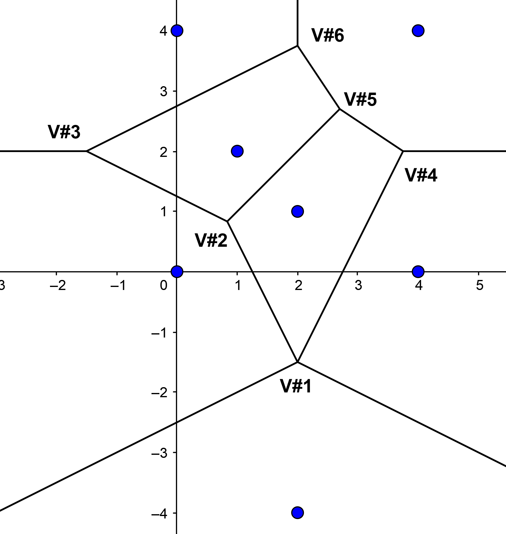
Voronoi diagram: Blue circles mark input data points, Voronoi diagram in black
6 Voronoi vertices: (2, -3/2), (5/6,5/6),(-3/2,2),(15/4,2), (27/10,27/10), (2,15/4).
The Voronoi vertex (2,-3/2) appears twice in the output with data point indices 1 5 7 and 1 2 5. This means that it is degenerate and is defined by the set of 4 input data point in positions 1,2,5,7 in the input file. I.e.. it is the centre of an empty circle through the four input data points (0,0), (2,1), 4,0), (2,-4). The other Voronoi vertices appear once each and are defined respectively by the data points with indices (i.e.. position in the input file) 1 2 3, 1 3 4, 2 5 6, 2 3 6 and 3 4 6. The Voronoi diagram has 5 rays
(2, -3/2) + (-2t,-t), (2,-3/2)+(2t,-t), (-3/2,2)+(-t,0), (15/4,2)+(t,0), (2,15/4)+(0,t)

For example, the first ray in the output appears:
V#1 R#1 B#1 h=0 data points 1 5* 7 det=64
0 -2 -1
This means that the ray (-2t,-t) emanates from the vertex V#1 defined by data points 1 5 7, namely (2, -3/2). The asterisk on index 5 indicates that the ray is defined by the data points with indices 5 and 7, namely (0,0) and (2,-4).

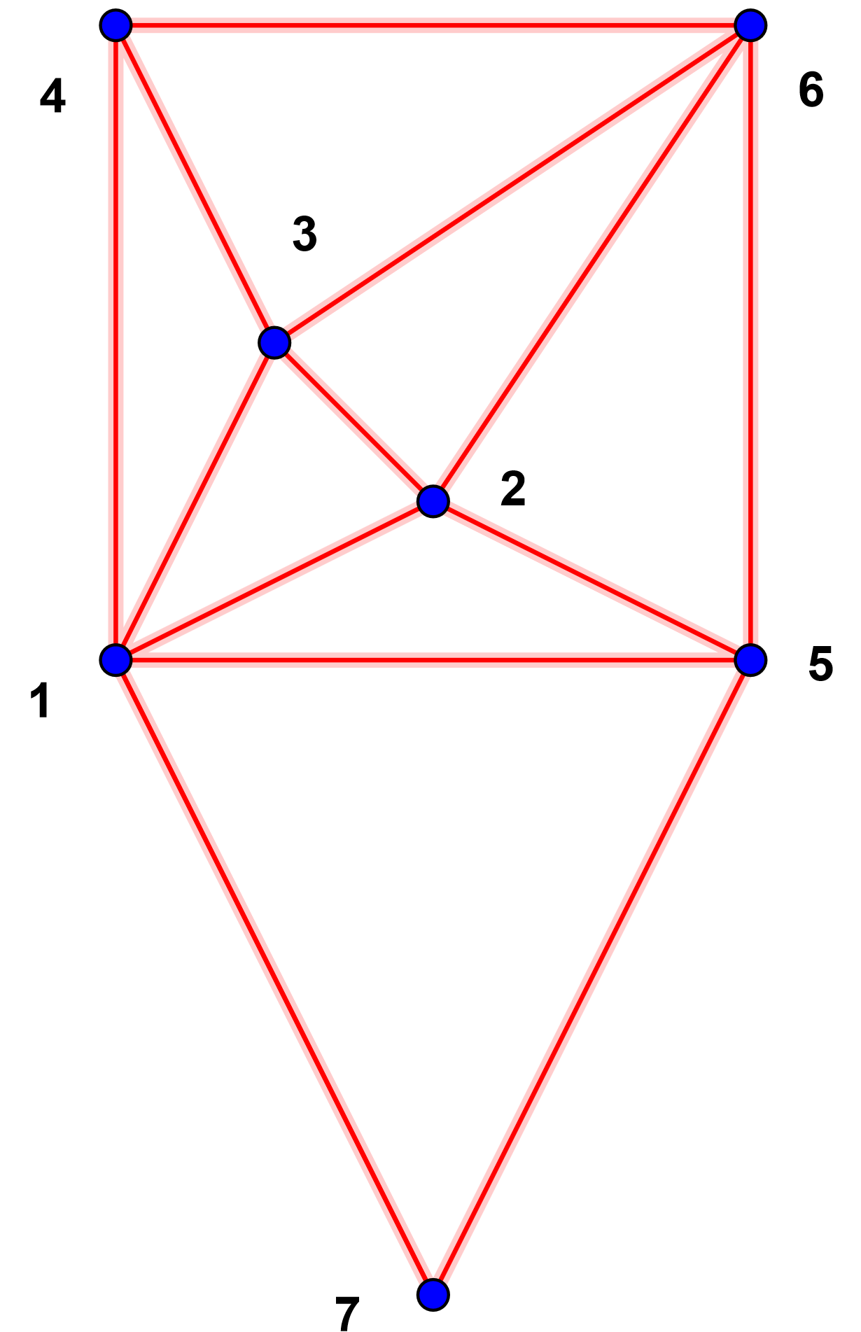
Delaunay triangulation Blue circles mark input data points, Delaunay triangulation in red.
Each of the 7 cobases defines a triangle in the dual: 157, 125, 123, 134, 256, 236, 346
Here each index refers to the line number of the data point in the input file.
Eg. 157 describes the triangle (0,0),(4,0),(2,-4)

Visualizations made using GeoGebra.

redund: extreme point enumeration and eliminating redundant inequalities (new options parallel version from v7.1)

minrep: finding a minimum representation of an H- or V-representation (new options parallel version from v7.3)

A convex hull problem that occurs frequently is to enumerate the extreme points (vertices) of a given set of input points. This problem is in fact much simpler than the problem of finding the facets of the given input point set. It can be solved by linear programming. The dual problem is to remove redundant inequalities from an H-representation. An input inequality is redundant if it can be deleted without changing the polyhedron. It is strongly redundant if it is not satisfied as strict inequality by any feasible point. A vertex/ray in a V-representation is strongly redundant if it is strictly interior to the convex hull.

An H-representation may contain "hidden linearities" or inequalities that are always satisfied as equations. A similar situation occurs in a V-representation where the convex hull contains a line. The minimum representation problem is to identify all linearities in an input file, output them explicity using the linearity option, and then remove any remaining redundant rows. The dimension of the input set is output at the end of the computation.

Redundancy removal can be obtained by using the lrs clone redund or by lrs via the redund/redund_list options described above.

A minimum representation can be obtained by using the lrs clone minrep or by lrs via the testlin (before the begin line) and redund/redund_list options.
mplrs can compute a minimum representation in parallel by use of the -minrep command line argument. Due to technical issues in the parallelization mplrs does not do redundancy removal without also computing a minimum representation.

The ouput will be streamed if the verbose option is included after the end line.
On each line *nr indicates non-redundant, *re indicates redundant, *sr indicates strongly redundant, and *li indicates linearity.

Usage:
(1) With options (allows partial redundancy checking for large inputs)

Add the redund or redund_list option after the end statement of a H- or V-representation.
Execute % lrs filename or %mpirun -np <procs> mplrs filename

If more than one redund/redund_list option is in the input file the last one read takes priority.

(2) Without options (complete redundancy check of all input lines, overidden by redund/redund_list option in input)

To remove input lines that are not vertices/rays from a V-representation or redundant inequalities from an H-representation use the command:

% redund filename or % mpirun -np <procs> mplrs -minrep filename

For example, using the file mit.ine from the distribution:

% redund mit.ine

*redund:lrslib v.7.1 2020.5.23(64bit,lrslong.h,overflow checking)

*Input taken from file mit.ine
mit.ine
*mulint : max(|a|,|b|) > 2147483647

*redund2 found - restarting
*redund:lrslib v.7.1 2020.5.23(128bit,lrslong.h,overflow checking)

*Input taken from file mit.ine
mit.ine
*row 75 was redundant and removed
*row 77 was redundant and removed
*row 89 was redundant and removed
--------------------------
*row 709 was redundant and removed
H-representation
begin
708 9 rational
36 0 0 -2 -2 -1 0 0 0
----------------------------

0 0 0 0 0 0 0 0 1
end
*Input had 729 rows and 9 columns: 21 row(s) redundant
*Overflow checking on lrslong arithmetic
*redund:lrslib v.7.1 2020.5.23(128bit,lrslong.h)

From this output we first see that redund tried 64 bit arithmetic but detected an overflow and reran with 128 bit arithmetic.
It found 21 redundant rows which were removed from the file.
The resulting output file can be used directly with lrs.
In fact, lrs works best if the input is non-redundant, see the section Redundancy vs Degeneracy.

Linearities

linearity k i₁i₂i ... i_k

The input file contains k linearities. If the input is a H-representation, the rows i₁ i₂i ... i_kof the input file are equations. For a V-representation, the rows with these indices should begin with zero in column one, and will be interpreted as lines rather than rays. Linearities defined on the input vertices of a V-representation are not defined, but the program will accept them and produce some output. Each of the indice i_k must be a distinct number between 1 and m. With an H-representation, linearities are useful for enumeration of vertices on a facet or lower dimensional subspace. For example the file:
cube_ridge
*cube of side 2 centred at the origin
H-representation
linearity 2 1 5
begin
6 4 rational
1 1 0 0
1 0 1 0
1 0 0 1
1 -1 0 0
1 0 -1 0
1 0 0 -1
end

causes vertices to be enumerated on the ridge which is the intersection of the two facets

x₁ = -1 and x₂ = 1

so the output is the pair of vertices

cube_ridge
*Input linearity in row(s) 1 5
V-representation
begin
2 4 rational
1 -1 1 1
1 -1 1 -1
end

Specifying linearities in this way will often produce redundancy , especially if the dimension of the problem is reduced considerably. As a preprocessing step, it is useful to apply to remove any redundancy by redund. In the case of the above problem the output produced by redund is:

cube
*Input linearity in row(s) 1 5
*row 2 was redundant and removed
*row 4 was redundant and removed
H-representation
linearity 2 1 2
begin
4 4 rational
1 1 0 0
1 0 -1 0
1 0 0 1
1 0 0 -1

and two redundant halfspaces were removed.

Redundant columns are closely related to linearities. If we examine the V-representation of cube_ridge above we can see that it is just a line segment in 3 dimensional space. Further, columns 2 and 3 are multiples of column 1. If lrs is applied to this file, the column redundancies give rise to two linearities, so the output will appear as the H-representation given above: geometrically the intersection of two planes (the linearities) with two half-planes (defining the endpoints of the line segment).

In general, the representation of the linearity space is not unique, however the one produced by lrs should be the same as that produced by cdd.

lrs timing and interrupts

     (for mplrs see here)

lrs handles certain signals unless it is compiled with the -DSIGNALS option. It is possible to interrupt lrs and get the latest cobasis, which can be used for restarting the program (useful if the machine is going down!)
        signal                     operation
        USR1                         print current cobasis and continue
        TERM                       print current cobasis and terminate
        INT (ctrl-C)                      ditto
        HUP                                      ditto
lrs also provides timing information unless it is compiled with the option -DTIMES.

For example, when hitting CTL-C when running

%lrs mit.ine

the following is obtained:

....
1 24 48 0 0 0 0 64 0
1 24 48 0 0 0 0 72 0

lrs_lib: checkpointing:
lrs_lib: State #0: (LRS globals)
restart 33 0 12542 8 634 640 641 678 704 725 726 729
integervertices 14
lrs_lib: checkpoint finished
4.476u 0.000s 0:04.49 99.5% 0+0k 0+0io 5657pf+0w

The restart and integervertices lines can be used to restart by adding them to the end of the mit.ine file:

0 0 0 0 0 0 0 1 0
0 0 0 0 0 0 0 0 1
end
restart 33 0 12542 8 634 640 641 678 704 725 726 729
integervertices 14

Now

% lrs mit.ine

*lrs:lrslib v.7.0 2018.6.14(64bit,lrslong.h,hybrid arithmetic)
*Input taken from mit.ine
mit.ine
*restart V#33 R#0 B#12542 h=8 facets 634 640 641 678 704 725 726 729
*lrs:overflow possible: restarting with 128 bit arithmetic

1 16 16 8 2 1 4 32 8
1 16 80/3 16/3 0 0 0 64/3 0
1 21 18 9/2 3/2 0 0 24 6
....

will complete the full run.

hvref/xref Cross reference listing between V- and H-representations               (new in v7.1)

This standalone hvref/xref makes a cross reference list between H and V representations.
The first step is to create a matching pair of representations using lrs/mplrs.
(The same steps can be used starting with a V-rep *.ext file)

First it is recommended to remove any redundancies from the input file using redund.

1. Add printcobasis and incidence options to cube.ine

% lrs cube.ine cube.ext        or   %mpirun -np <procs> mplrs cube.ext
% xref cube.ext

2. Edit the output file cube.ext.x to insert a second line that contains two integers

rows maxindex

where rows >= # output lines in cube.ext.x
      maxindex >= # input lines in cube.ine

or just use 0 0 and run as below, the output will tell you which values to use

% hvref cube.ext.x

Testing redundancy in projections

Given a polyhedron

P

with H-representation

b + Ax +By \ge 0

, the projection

Q

P

onto the

x

variables can be given by an H-representation

d + DX \ge 0

, where

x \in Q

if and only if there is some

y

such that

(x,y)

(x,y) \in P

D

can be computed by lrs/mplrs in fel mode by using the project/eliminate options.

Let

b + A_i +B_i \ge 0

be the

i

-th inequality in the H-representation of P.
This inequality is redundant in the computation of the projection

Q

if and only if deleting it does not change the projection.
This redundancy can be tested by computing the two projections and comparing them, a potentially very long computation.
lrslib contains an alternative way of testing this redundancy directly by use of an SMT solver without computing the projections directly.
This requires that an SMT solver such as z3 or cvc4 be installed.

projred is a script for performing this operation on one or more inequalities in an H-representation for

P

polyv is a C program for computing an SMT file to verify the redundancy of an inequality in computing a projection of

P

Error messages and troubleshooting

The most common error occurs from an incorrect input file specification, please check the section File Formats carefully. In particular, lrs does not check the type or number of input coefficients specified. After the line
m n rational
you must specify exactly m*n rational or integer coefficients. They are read in free format , but normally each input facet or vertex/ray is begun on a new line. See note for cdd users.

The following error messages are produced by lrs . They are arranged in alphabetic order.

Cannot find linearity in the basis

The linearity option was specified but a basis cannot be created. Check the linearity indices are all less than n-1 and are disitinct.

Data type must be integer of rational

lrs does not handle floating point data, change to integer or rational input.

Digits must be at most 2295 Change MAX_DIGITS and recompile (This message does not appear if the default gmp arithmetic package is used)

The digits option was specified, but the number of decimal digits is too large (the values shown here is for 64 bit machines). MAX_DIGITS (default 255) is the maximum number of array locations used for extended precision arithmetic. This value should be increased and lrs recompiled.

Invalid input: check you have entered enough data!

Usually means that end of file was reached before enough input data was read.

Invalid Co-basis - does not have correct rank

An attempt to restart from an invalid cobasis has been made. Check that the indices are entered exactly as they appear in the previous aborted run.

Maximize/minimize only valid for H-representation

LP operations can only be performed on H-representations.

No begin line

Input file does not contain a begin line. See File formats.

No data in file

The input file is incorrect, please check File Formats.

No feasible solution

The input is an H-representation of an infeasible system.

Starting cobasis indices must be distinct and in range 1 .. m

The startingcobasis option has been used, but the indices supplied were not valid: i.e. distinct numbers between 1..m.

Trying to restart from infeasible dictionary

An attempt to restart from an invalid cobasis has been made. Check that the indices are entered exactly in the order appear in the previous aborted run.

mplrs error messages

Error: lponly option not supported - use lrs!

The simplex method does not run in parallel

The following message may be produced when building lrs on macOS

OpenMP support not found, disabling OpenMP parallel build

Apple's Xcode compilers do not support OpenMP, so the build produced a single-threaded lrs. Multithreaded lrs can be built on macOS using e.g. gcc from MacPorts.

Hints and comments

H- vs V- representation

lrs is programmed to manipulate H-representations directly. A file presented as a V-representation is processed by lifting it to a cone in one higher dimension, which is treated internally as a H-representation. If the input file is a polytope which contains the origin, then the user has two options. Submit it as a V-representation and have it processed as just described, or submit it as a H-representation, and interpret the output as a list of facet inequalities rather than "vertices". Since this will not be lifted, it will be processed in a different way by lrs. Sometimes a degenerate V-representation may run more quickly as a H-representation, and sometimes more slowly. To decide which representation to use for a large problem, the user can run the estimates option and choose the representation with fewest estimated bases.

Redundancy vs Degeneracy

For an H-representation, an input is redundant if some inequality can be deleted without changing the polyhedron. It is degenerate if (in d dimensions) at least one vertex lies on d+1 or more facets. Similarly in a V-representation an input is redundant if some input point is not a vertex of the convex hull. It is degenerate if some facet contains d+1 or more input points. The options printcobasis and incidence give degeneracy information. Degeneracy causes pivot or triangulation based methods such as lrs to run slowly. Redundancy is one cause of degeneracy, but it can be avoided by pre-processing the input files. See section redund: extreme Point Enumeration and Redundant Inequalities for instructions on how to do this. This pre-processing is unnecessary if it is known that the input is non-redundant.

Even with redundant input removed a polyhedron may be highly degenerate. In distribution directory ine/metric there are many highly degenerate combinatorial polytopes. These are difficult problems for all vertex enumeration/convex hull programs that use pivoting, such as lrs. For example, the file cp6.ine is a polytope with 368 facets in 16 dimensions. It has 32 vertices, but computing these required the evaluation of 4,844,923,002 bases!(see Avis-Jordan, 2017)

Memory considerations

The strong point of lrs is that it does not save the output produced, so in theory it cannot run out of memory. With cache size one all memory is allocated at the beginning, so if lrs starts running it will not run out of memory. It is possible however that the number of digits required to do the calculations exceeds the amount specified on the digits option, or the default. In practice, this problem will also arise early in the computation. In any case, a message is printed and the calculation can be restarted. In order to improve performance, some dictionaries should be cached. The default of 10 can be overridden by the cacheoption. If the dictionary is in the cache it does not need to be recomputed when backtracking, reducing processing time by about 40%. Since the cache is allocated dynamically, a cache size that is too large can potentially use up large ammounts of machine memory.

Geometric Rays

A minimum V-representation of a polyhedron is a minimum set of vertices and rays such that each point in the polyhedron can be expressed as a convex combination of vertices plus a non-negative combination of rays. For the cube, if we delete the inequality
x₃ <= 1, i.e.. the line 1 0 0 -1 from file cube.ine, we get the output:
V-representation
***** 4 rational
1 1 1 -1
0 0 0 1
1 -1 1 -1
1 1 -1 -1
1 -1 -1 -1
end
indicating the polyhedron is the convex combination of 4 vertices and 1 ray. With the geometric option, we get the output:
V-representation
begin
***** 4 rational
1 1 1 -1
0 0 0 1 * 1 1 1 -1
1 -1 1 -1
0 0 0 1 * 1 -1 1 -1
1 1 -1 -1
0 0 0 1 * 1 1 -1 -1
1 -1 -1 -1
0 0 0 1 * 1 -1 -1 -1
end
This indicates that geometrically, the polyhedron has 4 parallel extreme rays (0,0,t) , one incident to each vertex. With the geometric option, all rays will be printed. Without the option, lrs tries to print each ray once, but in some cases duplicates will remain, see subsection Output Duplication.

Output Duplication

For degenerate inputs, pivot based methods for vertex/ray enumeration such as lrs may generate the same output ray many times. An output is only printed when it occurs with a lexicographically minimum basis. This removes all duplicate vertices, but rays may still be output more than once. This is due to the fact that duplicate geometric rays cannot always be detected without storing the output. Since V-representations are automatically lifted to a higher dimension, this will not happen for facet enumeration. Unless the allbases option is specified, lrs makes checks in order to remove duplicates. A warning message is produced when duplicates may occur in the output. They can be removed using the program buffer.c. Two important types of input never produce duplicate output: polytopes (i.e. bounded polyhedra) and cones (i.e. polyhedra where the origin is the only vertex).

Acknowledgements and References

I would like to thank many people for helping with this implementation project. Komei Fukuda encouraged me from the start, collaborated in designing the file formats, and provided many suggestions for improving the code. Debugging would have been almost impossible without the use of his program cdd as a benchmark. David Bremner implemented memory allocation, cacheing and signals. Ambros Marzetta demonstrated the importance of cacheing and lrslong is based on his earlier implementation of this as prs_single. Jerry Quinn coded the integer divide routine. Bug reports were provided by many users, for which I thank them. In particular Gerardo Garbulsky's extensive use of earlier versions suggested many refinements and Andreas Enge helped debug the volume computation. Tallman Nkgau contributed fourier.

D. Avis, lrs: A Revised Implementation of the Reverse Search Vertex Enumeration Algorithm, http://cgm.cs.mcgill.ca/~avis/doc/avis/Av98a.ps
In: Polytopes - Combinatorics and Computation, Ed. G. Kalai and G. Ziegler, Birkhauser-Verlag (2000) 177-198.

D. Avis, "Computational Experience with the Reverse Search Vertex Enumeration Algorithm," Optimization Methods and Software, (1998 (to appear)). http://cgm.cs.mcgill.ca/~avis/doc/avis/Av98b.ps

D. Avis, D. Bremner, and R. Seidel, "How Good are Convex Hull Algorithms?," Computational Geometry: Theory and Applications, Vol 7,pp.265-301(1997). http://cgm.cs.mcgill.ca/~avis/doc/avis/ABS96a.ps

D. Avis and L. Devroye, "Estimating the Number of Vertices of a Polyhedron," pp. 179-190 in Snapshots of Computational and Discrete Geometry, ed. D. Avis and P. Bose, School of Computer Science, McGill University (1994). http://cgm.cs.mcgill.ca/~avis/doc/avis/AD94a.ps
In: Information Processing Letters, (2000) V. 73, pp. 137-143.

D. Avis and K. Fukuda, "A Pivoting Algorithm for Convex Hulls and Vertex Enumeration of Arrangements and Polyhedra," Discrete and Computational Geometry, Vol. 8, pp. 295-313 (1992). http://cgm.cs.mcgill.ca/~avis/doc/avis/AF92b.ps

D. Avis, K. Fukuda and S. Picozzi, "On Canonical Representations of Convex Polyhedra", Mathematical Software, ICMS 2002, Ed. A. Cohen, X-S Gao, N. Takayama, World Scientific, pp.350-360 (2002) http://cgm.cs.mcgill.ca/~avis/doc/avis/AFP02a.ps

D. Avis, G. Rosenberg, R. Savani, B. von Stengel, "Enumeration of Nash Equilibria for Two-Player Games", Economic Theory 42(2009) 9-37 pdf

D. Bremner, K. Fukuda and A. Marzetta, Primal-Dual Methods for Vertex and Facet Enumeration, 13th ACM Symposium on Computational Geometry SCG 1997, 49-56. http://www.cs.unb.ca/profs/bremner/pd/